
It’s easy to add a line break when you’re typing in an Excel worksheet. Just click where you want the line break, and press Alt + Enter. But how can you add a line break in an Excel formula?
Line Break in Excel Text
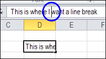
Here is an example of adding a line break in Excel text.
- The cursor is positioned where the line break should be added.
- Press Alt+Enter
- Press Enter, to complete the entry and move to another cell
Wrap Text Added Automatically
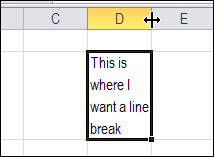
When you press the Enter key to complete the entry, the line break appears, and Wrap Text is automatically added to the cell.
You might have to adjust the column width though, because the text won’t flow into the next column.
Add a Line Break in a Formula
It’s not quite as easy to add a line break in a formula, but it’s possible!
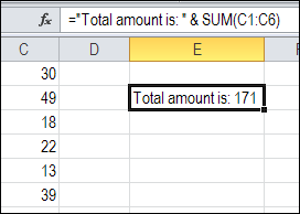
Here is a formula that shows text, combined with the sum of the values in C1:C6
=”Total amount is: ” & SUM(C1:C6)
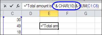
To add a line break between the text and the total amount, use the Excel CHAR function, with the number 10. The “&” operator is included too, to join the line break character to the other text in the formula.
=”Total amount is: ” & CHAR(10) & SUM(C1:C6)
Turn on Wrap Text
After you add the line break, and press Enter, you might see a strange little box, where the line break should be.
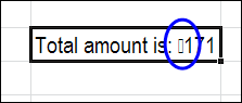
The Wrap Text feature isn’t automatically turned on, when you add a line break in a formula. You’ll have to turn it on yourself.
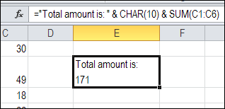
Select the cell with the line break in the formula, and on the Ribbon’s Home tab, click the Wrap Text command.

Then, you’ll see the line break in the cell, instead of the little square.
Video: Find and Replace Line Breaks
Watch this short video, to see the steps for adding a line break in a cell that contains. Then see how to find the line breaks in Excel, and replace them with space characters.
To get the Excel workbook, with the Add or Remove Line Breaks in a Cell in Excel example, go to the Excel Line Breaks page on my Contextures site.
__________
I have a formula that grabs data from page 1 in a workbook I have to create various printed results.
=IF(ISBLANK(DATA!$C1),””,DATA!$G$1&DATA!$C1&DATA!$G$2)
The result would be “AB12345C, where DATA!G1 would be AB, DATA!C1 would be 12345 and DATA!G2 would be C
I want to insert a space between the C1 and G2 cells so that the result in the cell is this…
AB
12345C
I have text wrapping on. I’ve tried to insert the “CHAR(10)” into various parts of the formula. Any questions?
PS. Reason being for so many $ in the formula is that those cells are the prefix and suffix of a serial number generator I made, only one cell changes so this formula will be used multiple times with only one cell data varying.
Any idea?
Try setting vertical format to Justify on the cells that will display this information. Right Click -> Format Cells… -> Alignment -> Vertical = Justify.
Doesnt work if you have an equation to continue the stacking of text in a single cell.
Thanks, Char(10) worked…
Thank you. May God Bless you.
CHAR(10) worked like a champ..Thanks a lot guys!!
great stuff – as always. Thank you Debra!
@Rich, thank you!