
It’s finally summer, and you need to stay cool, even when you’re using Excel. Here’s an energy-efficient and fast way to find and delete Excel rows. You can select several rows that contain similar data, and delete them all at the same time.
Find All the Data
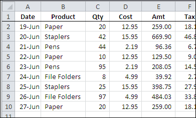
In the worksheet shown below, there is a list of products sales, and a few of the records are for paper sales.
I’d like to delete those paper sales rows, without having to sort the worksheet, or spend a long time manually selecting the rows.
Find the Paper Rows
To find all the Paper sales rows, I can use the Excel Find command. Here are the steps to do that:
-
- On the Ribbon’s Home tab, click Find & Select, and then click Find.

- In the Find and Replace dialog box, type “paper” in the Find What box.
- Click Find All, to see a list of all the cells that contain the text, “paper”
- Select an item in the list, and then press Ctrl+A, to select the entire list. That will also select all the “paper” cells on the worksheet.

Delete the Selected Rows
To delete the entire row for each “paper” cell that was found, follow these steps:
- On the Ribbon’s Home tab, click Delete, and then click Delete Sheet Rows.
All the selected rows will be deleted, and the other product orders remain on the worksheet.

Video: Find and Delete Excel Rows
To see the steps to find all the instances of a word, and delete the selected rows, watch this short Excel video tutorial.
More Find and Replace Examples
See more ways to use the Find and Replace commands in Excel, on my Contextures website.
Also, see how to select rows based on their conditional formatting colour, and delete the filtered rows. This example uses a list in a named Excel table.
___________
Thx, its very useful for my works.
Why not just put a filter on paper and delete the rows. I think that’s quicker.
Really, hats off to you; I save a lot of time with using this technique. Debra Dalgleish 🙂
Thank you very much :)!
This is fantastic for word searches, but what if you want to delete rows of cells containing dollar amounts below $600.00? I was able to conditionally format the spreadsheet to highlight figures under $600.00 but can’t find a way to mass delete those that have been highlighted. Your help is appreciated.
@Mrs. B, instead of using this method, you can apply a filter, then delete the filtered rows
Assuming that your list is in a named Excel Table (http://www.contextures.com/xlExcelTable01.html), follow these steps
Make a backup copy of your file first — just to be safe.
1. Click the arrow in the heading for the column where you applied the conditional formatting
2. In the drop down, click Filter by Color, and select the color that you used.
3. Select the colored cells, and on the Ribbon’s Home tab, click the arrow under the Delete command
4. Click on Delete Table Rows.
5. Remove the filter, and check that all the other rows are still okay, and the colored cells have been deleted.
If it doesn’t look right, click the Undo button, or press Ctrl + Z to undo the deletion.
it is quite simple. It saved my lot time. Thanks for sharing this.