If you select a cell in a pivot table and click the Chart Wizard button on the toolbar, a default pivot chart is created, on a new chart sheet.
Sometimes you might want to step through the Chart Wizard, so you can set the options as you create the pivot chart.
Use the Chart Wizard
If you follow the steps below, you can use the Chart Wizard, instead of creating the default pivot chart.
- Select an empty cell on the worksheet, away from the pivot table and any other data.
- On the Excel toolbar, click the Chart Wizard button.
- In Step 1 of the Chart Wizard, select a Chart type and Chart sub-type, then click Next.
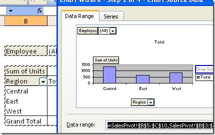
- In Step 2 of the Chart Wizard, click in the Data range box, and select any cell in the pivot table.
- The entire pivot table will be automatically selected, and its address will appear in the Data range box.

Complete Chart Wizard Steps
Next, complete the remaining Chart Wizard steps, selecting the options you want
When you’re done, click the Finish button, to create the pivot chart.
Chart Wizard Note
If you select a pivot table as the data range, you can’t return to Step 2 of the Chart Wizard.
To use a different data range, you’ll have to start over, and create a new chart.
__________________
