
When you were first learning how to use Excel, you quickly discovered the basic Excel functions, like SUM, COUNT, MIN, MAX, and AVERAGE. Now you’re ready for advanced calculations, like how to find MIN IF or MAX IF in Excel.
Beyond the Basics with MIN IF
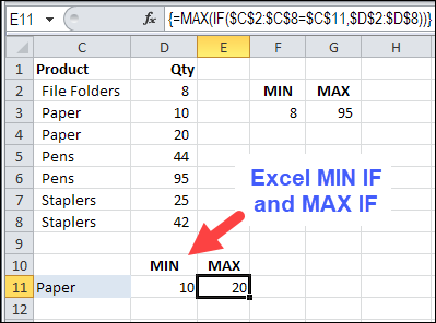
In this example, we want to see the MIN and MAX for a specific product. There is a SUMIF function and a COUNTIF function, but no MINIF or MAXIF.
- [Update]: In Excel 2019, and Excel for Office 365, you can use the new MINIFS and MAXIFS functions. There is more information on the MIN and MAX page on my Contextures site.
So, we’ll have to create our own MINIF formula, using MIN and IF. I’ve selected a product in cell C11, and the formula will be built in cell D11.
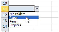
To make it easy to select a product, I created a drop down list of product names, by using data validation.
NOTE: You can also calculate MIN IF and MAX IF with Multiple Criteria
MIN IF Formula
The formula starts with the MIN and IF functions, and their opening brackets:
=MIN(IF(
Next, we want to find the rows where the product name matches the product in C11:
- Select C2:C8, where the product names are listed
- Type an = sign
- Click on cell C11
=MIN(IF(C2:C8=C11

Next, select D2:D8, where the quantities are listed. If the product name matches, we want to check the product quantity
=MIN(IF(C2:C8=C11,D2:D8

To finish the formula:
- Type two closing brackets
- Then press Ctrl+Shift+Enter to array-enter the formula.
=MIN(IF(C2:C8=C11,D2:D8))

NOTE: If you plan to copy this formula down a column, use absolute references to the product and quantity ranges:
=MIN(IF($C$2:$C$8=C11,$D$2:$D$8))
Array Entered Formula
If you select cell D11, and look at the formula in the Formula Bar, there are curly brackets at the start and end of the formula. Those were automatically added, because the formula was array-entered (Ctrl + Shift + Enter).
If you don’t see those curly brackets, you pressed Enter, instead of Ctrl + Shift + Enter.
To fix the formula:
- Click in the formula bar (it doesn’t matter where you click within the formula)
- Press Ctrl + Shift + Enter.

Create a MAXIF Formula
To find the maximum quantity for a specific product, use MAX instead of MIN.
=MAX(IF(C2:C8=C11,D2:D8))
or use absolute references for the product and quantity ranges:
=MAX(IF($C$2:$C$8=C11,$D$2:$D$8))
And remember to press Ctrl+Shift+Enter

Multiple Criteria for MIN IF or MAX IF
These formulas have only one criterion — the product name. If you’re ready for the next challenge, you can also calculate MIN IF and MAX IF with Multiple Criteria
- [Update]: In Excel 2019, and Excel 365, you can use the new MINIFS and MAXIFS functions. For more information, go to the MIN and MAX page on my Contextures site.
Watch the MIN IF or MAX IF Video
To see the steps for creating MIN IF and MAX IF formulas, watch this short Excel video tutorial. The sample file for this video can be downloaded from my Contextures website, on the MIN and MAX page.
________________________

________________
Min IF or Max IF is going to be very useful to me in the near future.
Wow, that’s very cool, Debra. Thank you!
I like it!
can use in VBA:
Range(“D11?).FormulaArray = “=MIN(IF(C2:C8=C11,D2:D8))”
Thanks VERY much!!! I spent about 4 hours trying to work out how to take the highest number from a large list of numbers if the first three numbers were “x” and with the help of your webpage, I got it sorted. Thanks again!!!!
You’re welcome! Thanks for letting me know that the instructions helped you.
Great article, many thanks!
Hi thank you for great article. Is it possible to combine more conditions? I tried to put and function inside if but it didnt work. Can you please help me?
seems that it cannot run in 2003
I agree, is there a way to make it work in Excel 2003?
CTRL + SHIFT ENTER
That formula is not working. I even tried the exact same information. I am using excel 2010. It gives me error: #value!
@Dora, remember to press Ctrl+Shift+Enter to array-enter the formula.
It won’t work correctly if you just press Enter
Thanks Debra!! I forgot that.
Hi. I keep getting the #Num error when using this. Do you know why?
Brilliant! Am at a coal mine in the middle of nowhere going through some data, and found your website in a frantic google search while sitting outside in the carpark with 1 bar of signal. Lifesaver. Cheers for the humourous instructions.
@George, thanks, and I’m glad you found the solution when you needed it.
Thank you very much, certainly useful and much simpler than I expected!
PRODUCT RED GREEN BLUE MAXIMUM
A 0 10 0
B 12 0 0
C 0 0 9
How I will get the maximum nos by using if formula.
THANK YOU SOOOOOOO MUCH!!!! I spent hours trolling around the internet trying to find a MAXIF-like formula. This website saved my PowerPoint deck (and my tail)….lol
EXCELente !!! muchas gracias
It’s a shame such a normal (and useful) function as this still has to be done with the memory-hogging Array formula. I guess Microsoft won’t get around to adding it as a normal function until Office 2025?
This explanation was a major boon to my worksheet development. Thanks so much!
Thanks for this; is there anyway to know in advance whether I will need to convert formulas in excel into array formulas. Not 100% sure of when a formula should be an array vs a standard formula.
ty in advance
That’s great, but I’d like to take it a bit further. I’d like to combine the small/large functions with an if condition. Basically, I want to find the top/bottom 20 values in a column, given that 2 other conditions hold true. Does that make sense?
I can obviously do this with a pivot table using filters, but prefer to avoid having to update them each time. Thanks.
THANK YOU SO MUCH…………!!!
I have run into two issues…maybe someone can help.
1) The calculations take a long time when adding this formula.
2) if there is a #N/A in the data, it comes up with #N/A instead of ignoring it
Thanks!
Hi,
You probably found an answer to this as it was a few months ago, but if not, use:
=IF(ISERROR(insert debra’s fantastic formula here),””,insert debra’s fantastic formula again)
Why not just use:
=IFERROR(insert Debra’s fantastic formula here),””)
This way you don’t have to repeat the resource consuming Debra’s fantastic formula…
Very valid issue where this formula stumbles is that if the cells are blank or null, then it returns the min value as zero, and I solved it like this. It ignores all ZERO blank NA values and calculates perfectly:
=MIN(IF($U$2:$U$927>0,IF($B$2:$B$927=B157,$U$2:$U$927)))
This is a great method and it seems to work very well. I have a situation where the data is not arranged in a “vertical” array. By this I mean the records are listed column-wise, not row-wise. Unlike the capability of the built-in function =averageif() which works both ways, I can’t seem to get this method to work in an array where new records are added horizontally in columns.
Can you verify if this is true?
thanks, -doug
Thnk you evry much. I’ve been working on this for quite a while, but this is an easy solution. Thanks for putting it online for everyone! I’m sure you’ve helped a lot of people, most people dont post a thankyou…
I love thinking out of the box! Great explination and very very useful!!
Thanks for wonderful explanation,,, its really informative!!!!
Thanks – this array function is working well for me as a substitute for MAXIFS in my local file. However, after I got is all tested and working, I posted these changes into the live file which is a shared Excel file on my company’s internal network server. Turns out, it does not work well in a shared file. When one tries to copy, or insert rows, Excel 2007 returns this error:
Error 1004:
Cannot copy or move array entered formulas or data tables in a shared workbook.
Does anyone know of any way to do MAXIFS without using array formulas? e.g. without using Ctrl+Shift+Enter?
Thanks,
Jeff
Great article, thanks so much, saved me a lot of time.
So I have used the MIN IF many times now, but for the first time I have gaps in the data, while the min function would traditional ignore blanks, the MIN IF inserts a 0. Certainly something to mindful of but does anyone know a work around?
Debra:
This explanation is excellent and easily understood. More importantly, it has helped me immensely with several projects which would have been quite complicated without your great help.
This is great and works well. How can you change the formula to look up the Product column and then list each product and its corresponding highest or lowest value?
Thus you don’t have to referenc cell C11 i.e. here is a list of all my products show me the max/minmum for each.
Thank you!
Perfect! Just what I was looking for.
Cheers
I HAVE IN A1 MONTH LIST , B1 AMOUNT , C1 AMOUNT I NEED TO MAKE D1= IF A1=1JAN TO 30 MARCH AMOUNT IN B1 IF A1= 1 APRIL TO 31 DEC =C1
Hi,
If I enter “paper” in C12 and “pens” in C13, can I copy the array formula down? Don’t seem to be able to do that – it still seems to link only to C11 (even if I remove the absolute reference)? Any help?
I am having this same issue. The cell reference copies down to all other rows as if it was an absolute reference. I haven’t found a solution to this yet.
Thank you for this post. That was exactly what I needed.
Thks again for sharing.
Can I use this formula with 2 conditions?
I try = MIN(IF(AND(…, …),…)) –> Ctrl+Shift+ENter but it doesn’t work 🙁
Please advise.
Thanks,
Use =MIN(IF((..=..)*(..=..),..)) –> Ctrl+Shift+Enter
Thanks!! This solved my problem perfectly 🙂
thank you that was easy and very helpful 🙂
Thanks, works great. I learnt something new today. The only issue is it’s a bit processor heavy when dealing with large spreadsheets. Still I suppose there is no way round that. Thanks again.
An easier-to-remember way to achieve this is using the SUBTOTAL formula. E.g. SUBTOTAL(5,filteredRange) will give the MIN value, and SUBTOTAL(4, filterRange) will give the MAX value.
I’ve spent years dealing with donor ids and giving histories by gift and having to sort to only show the last gift. MAXIF would have saved me countless hours and headaches. Thanks so much!
Thank so much
It fails if you are using tables in 2013, eg: =MAX(IF(A2=Tx_Hist[@Description],Tx_Hist[@[Prd_date]])). It works OK for the first 2 rows, then returns zero for the rest of the table.
wow thats a million this saved my time a hell lot!!!
Thanks for having such an awesome tutorial on MIN IF and MAX IF! It works perfectly in 2010!
I want to extend this formula “one step” further. That is in column E let’s say I have first names listed. So instead of finding the maximum value 20 for “paper”, I want the formula to return the name in column E. Specifically cell E4 in the above example.
I have found formulas that will return E4 if it is a number, but I get an error if the cell in non-numeric.
This was very helpful, worked like a charm! saved me so much time, thanks you so much, God Bless you!
Very helpful. This formula is the best. Thank you so much 🙂
Thank you so much for the Max(If) formula. It works perfectly when the data is in the same sheet. However, I have data in different sheets, and got back an error #REF!
For example I have a sheet with 50 states listed down the page in column A, number of employee in column B and $Amount in column C. There are 25 sheets for different companies. I want to find the Max $Amount for each state among the 25 companies if number of employee is > 1000.
Does the Max(If) works when your data is in different sheets? Thank you so much for your help on this.
from the sheet where you get your data, there is a #REF! as your data.
Simply use sort and check if there is a #REF! from your list.
check if there is a #REF! from your data. It is possible to use even if the data is from a different file.
Very helpful. Thank you so much!
Thanks for the MaxIF suggestion. I needed to find a the maximum value less than 0 in an array with 2000+ entries. I wasn’t looking forward to 2000+ IF statements then using MAX on these to find the answer. Several of the lookup type functions were checked and didn’t work out.
The key insight was to view this as array entered and either add the {} or use Ctrl+Shift+Enter.
Your approach took 1 simple statement.
Thanks,
MarkinID
Debra Dalgleish you rock thank you. You instructions were clear and precise. I was able to duplicate this the first time.
Thanks, Jeanie! Glad it helped you, and thanks for letting me know.
Works a dream – many hours saved.
Hi,
Can we apply a formatting condition in this formula somehow?
If I have a row of dates and the first four dates a highlighted green. How can I identify that last green date/cell?
Thank you!
Thanks a lot, information was really useful & I could able to use it for my work. I could able to write formula but missing {} brackets, but key trick mentioned was magic for me.
Best Regards,
Sandeep
Many thanks, your article is still helping people after more than 3 years! 😉
Thank you for the post! I applied the Min IF function on a large dataset it returns values for about 35000 rows but fails beyond that. Does anyone have any good suggestion how to extend the rage of the function?
Thank you very much for the guidance
It really helps!
Thank you very much for this explanation. It worked perfectly. Can I ask a question just for lerning purposes: why doesnt it work with out presing ctrl shift enter?
Excel treats formulas as array formulas only when Ctl+Shift+Enter is pressed. In order to do a min of an array, we need to use array formulas. I was looking for a way to avoid array formulas, as they sometimes slow Excel down (if used in thousands of cells). So far, it looks like array formula is unavoidable. This method shown here is the only method I have been using. Thanks.
I don’t like array formulas, because I design spreadsheets for other people to browse and look at data sets from different perspectives. The danger with array formulas is someone can click on your cell and the array designation will disappear. Just something to be aware of if trying to make a fool-proof spreadsheet.
“If you make something fool-proof, the world will create a better fool”
Thank you very much.
It was very helpful.
This is useful! Thank you!
I have a problem with Excel 2007 whilst trying to total max and min in a row for weather recording. The conditional format works on MAX on the row between B34:Y34 but the MIN function does not. I have tried everything I can think of, but nothing works. The conditional format works on columns but not across rows! Do you know why? Would welcome your advice.
Thanks for this. Worked like a charm. I subscribe to PPP, so I’m not surprised at all that I found great advice here. PPP is a great product.
@TJF, thanks, and I’m glad you like the Pivot Power Premium add-in too!
Thank you Debra! I liked the commentary perhaps even more than the actual advice (which was great). Rocks and tree stumps!
@david, thanks, I’m glad you liked it! 😉
Debra,
Thanks for posting this! I learned a ton not just on nesting functions but about arrays in formula. This opens up a whole new world to me!
Thanks Brus!
This solved one of my biggest headaches…where we have columns of values, but they alternate (e.g. North, East, South, West), grouped for different years and I want to display, on the same row (e.g. “sales”). Before I had tried to do this with named areas, but that was tedious as each row had to have its own named areas, and formulas couldn’t be copied.
It’s surprising MS hasn’t incorporated this as a standard function already!
Thanks;)
Awesome;)
Emp ID Emp Name PRJ-1 Start Date End Date
12345 Everest A 12-Aug-15 28-Aug-15
12345 Everest B 31-Aug-15 16-Oct-15
12345 Everest C 6-Jul-15 31-Jul-15
12345 Everest d 3-Aug-15 11-Aug-15
using above example how to extract the Min and Max function by using Vlookup for the same Empid
its knowledge full thanks
hi, how i do minif for value > 0 ?
I am able to create an array for one record, but need to copy it to many records. I tried highlighting all cells, editing the first and pressing Shift-Control-Enter. The first record is correct, but all of the formulas reference the first. I made sure that the formula only included absolute references for the ranges, not the conditions.
Help please!
=MAX(IF(‘Meeting Log’!$B:$B=’Client Summary’!B3,IF(‘Meeting Log’!$D:$D=”Held”,’Meeting Log’!$C:$C)))
Really useful, thank you! Myself and a colleague wasted the best part of an hour trying (and failing) to formulate this ourselves.
Worked perfectly, thanks!
Hello,
I have a question . Does this Formula work if there are references to another sheet ?
Thanks a Lot!
@Bastian, what happened when you tried it?
Actually I have tried the same figures in Excel 2007, it gives me error as#Value.. I am not able to make out where I am wrong here.. I used same database as shown above. Please help..
Make sure to press CtrlShift+Enter after entering or editing the formula
If you just press Enter when you complete the formula, it will show an error.
I am trying to repair a max(if(… formula where someone sorted the file without having absolute references where they belonged. Now everytime I try to repair a reference the only thing I get back is a 0. I am actuall bringing back the max date entered into a second tab. the cell comes back as 1/0/1900. Every cell comes back this way without giving me the latest date entered in the range. Does anyone have insight on this? I have pressed CtrlShift+Enter. I have tried formatting the lookup employee number making both the reference and the lookup lists be formated to a number. I don’t understand why it is not working.
That was really helpful I’ve been searching for it for ages :)))
Would you please do me a favor and explain why it is not working without array-entering it?? what’s the logic behind array-enter???
I need to understand ^_^
Thanks
Hey, thanks!! Helped. Can you please share the logic of why Cntrl+Shift+Enter and not just Enter works. I tried typing in the “{” signs with the keyboard rather than “Cntrl+Shift+Enter”… that did not work..
Brilliant! Thank you! (As always someone has the answer to what you need in excel, it’s just a question of finding it!)
Great example! Thanks a lot!
Hi,thank you very much. I was able to do the same with LARGE function. The trick was to use Ctrl+Shift+Enter to array array-enter the formula and it worked as expected. Very kind of you to share this knowledge with us.
I’m having difficulties with the results as I have in my list dates instead of numbers, as you know dates are numbers as well. Also I have my list of variables ea A,B, C, D etc in which for A I have fro example 4 different dates and for B could be 2 different dates and C just one date and D could be 2 or 3 dates, now when applying the formula it brings for eac case the max date from the whole list not from the specific variable, can anybody help with this?
Hello Debra,
I am trying to return min and max dates but I keep getting 1/0/1900 as my date which is not accurate. Do you know what might be causing this?
Hi,
I have a file with a sheet (“Donations”) containing a list of donations. Each donor is tagged with an alphanumeric UID ending in letters which correspond to various criteria – an A in their UID means they’re an Active Member, X for ex-trustees, P for prospect donors, V for volunteers; a UID can have multiple letters if they meet more than one of those criteria.
Column B of my Sheet1 lists each of the unique criteria codes (P, V, X….). On the Donations sheet column A lists the UIDs and column D lists the donation given by each donor.
I can easily work out the total and average donation amounts for each of those criteria codes (where I’m looking up the criteria code in row 34):
=SUMIF(donations!A:A,”*”&B34&”*”,donations!D:D)
and
=AVERAGEIF(donations!A:A,”*”&B34&”*”,donations!D:D)
But how do I work out the minimum and maximum amounts given by each code? I’ve tried:
{=MIN(IF((donations!A:A=”*”&B34&”*”),(donations!D:D)))}
but it just gives me a zero value. I use Ctrl+Shift+Enter since it’s an array formula.
Can you help?
Love your work by the way.
Thanks!
You can use the SEARCH function to check for the letters, and ISNUMBER to test if a number was returned.
This is an array formula, so press Ctrl+Shift+Enter
=MIN(IF(ISNUMBER(SEARCH($B34,Donations!$A$2:$A$6)),Donations!$D$2:$D$6))
Same thing for MAX
=MAX(IF(ISNUMBER(SEARCH($B34,Donations!$A$2:$A$6)),Donations!$D$2:$D$6))
hi, i dont know why, but even if i copy the formula from this page, click ctl shift and enter it doest give me values, excel locks me asking if i am not trying to type formula.
and it show the pop up, just after i put ” ,” after =min(if(A1:A5;A7, please help
Depending on your regional settings, you might need to use a semi-colon as a separator, instead of a comma
=MIN(IF(A1:A5;A7;
How could we adjust this formula to grab the minimum value that is greater than zero?
Hi chris, use the small function: =SMALL(array,k) where =SMALL(array,1) = same as =MIN(array) as k is the k’th smallest
=SMALL(IF($C$2:$C$8=$C$11,$D$2:$D$8),2) <- if your next figure is above 0.
else if you have multiple zeroes try:
=SMALL(IF($C$2:$C$8=$C$11,$D$2:$D$8),countif($D$2:$D$8,0))
Thank you very much
Thanks a bunch. You saved my day!
Help. I used {=min(if(…. on a 2 column table with 1450 rows of data. All the criteria in coulumn A was = the date I was searching on, but result was NOT the actual minimum value of the table. I ran {=count(if(… to doublecheck that all rows are being considered, and it returned 1200 (not 1450). Any reason you can think of why {=min(if(… isnt considering all rows?
sorry, was my bad. dataset was corrupt. the function/array worked perfect once i fixed it. 🙂
Thanks for the update, and I’m glad you got it working
why this formula [=MAX(IF(A:A=11,B:B))] not work on a sheet containing 10000 records
I want minimum number from 0,1,2,3,4,5,3,0,4,6,1,5,0,1,0,5 where minimum> 0
I want to grab a text from the minimum value of 3 , Eg
a=1
b=2
c=3
d=1
min of a,b,c & d is 1 so return “a” ( if you have many in common of select from a priority list)
Thanks!
Can I use MIN and ISNUMBER? i want to sum a range only if a cell contains numeric value. please assist
Thank You So Much
Very very useful tip, save me tons of time ! Thank you so much Debra !!
please solve below problem
If in one excel have 1 to 100 code and in another excel also have the same code but with a different order, how we cross-check in both excel having codes