Contextures Black Friday Sale 2014

Happy Black Friday! If you celebrated Thanksgiving yesterday, I hope you enjoyed time with your friends and family, and are ready to do some shopping today.

To celebrate Black Friday, the busiest shopping day of the year in the USA, you can buy my popular ebook kit – Excel UserForms for Data Entry – at 50% off today. So, instead of the regular price of $30 US, you can get the kit for only $15 US. The price will be reduced automatically – you don’t need to enter a coupon code.

[Update: This product is no longer available]

The special price ends tonight (Nov. 28, 2014) at midnight, Toronto time (Eastern time zone).

Click here to see the details, and grab a copy of this awesome kit.

Excel UserForms for Data Entry

Continue reading “Contextures Black Friday Sale 2014”

Convert Currency With Different Separators

Happy Thanksgiving, if you’re celebrating today. Tomorrow is Black Friday – the biggest shopping day of the year, in the USA. Up here in Canada, we celebrate the day too, so I’ll put one of my Excel products on sale for the day. Remember to check this blog tomorrow, to get the coupon code.

If you’re doing your shopping around the world, you might end up with a worksheet filled with amounts in a different currency. Let’s see how Excel can help with that problem!

Continue reading “Convert Currency With Different Separators”

Ignore Blank Cells When Pasting

Last week, I was working on a client’s file, and we wanted to get any new information from an update file, and paste it into the current record.

Both files were set up with the same columns, but the update file only had a few of the fields filled in. We could have used a macro to loop through the fields, grab any new information, and paste it to the current record. However, that would be a slow way to update the records, especially in a large file.

Continue reading “Ignore Blank Cells When Pasting”

Excel Roundup 20141117

In this Garage Series episode, Power BI and Excel go to Spain, to expose data patterns in past matches between Real Madrid and FC Barcelona.

“By combining historical El Clásico and player data, outside forces like temperature, humidity and moon phases, Jeremy tries to predict the outcomes and puts these predictions to the test among fans in Barcelona.”

They didn’t use good hair as one of the factors, but they predict 2-1 for Madrid, in the Oct. 25th match. (The final score was 3-1 for Madrid.)

You can watch the video below, or on YouTube: Power BI takes on El Clásico

Continue reading “Excel Roundup 20141117”

Create Custom Reports From Pivot Tables

If you’re a pivot table fan, like I am, you know how quick and easy it is to summarize a massive amount of data, with just a few clicks. You can show sums, counts, averages, and other totals, without using any fancy formulas.

In the screen shot below, the pivot table is summarizing income and expenses, and there is a Slicer at the top left, for quick filtering.

getpivotdatarg01

Formatting Restrictions

As wonderful as pivot tables are, they do have some limitations, and you might not be able to get the layout exactly the way you need it. In the screen shot below, you can see a P & L statement, based on the same data as the previous pivot table.

You’d never be able to get the pivot table in exactly this layout, with its blank rows, and formatting, and there are additional formulas at the right side too.

getpivotdatarg02

Create a Custom Report

Roger Govier is a pivot table fan too, and he has created a solution for building his own custom reports, like the P & L statement shown above. Roger creates a pivot table first, and then he uses the GetPivotData function, to pull specific data into his custom layout.

In the formulas, Roger uses cell references to the row and column headings, so he just has to create one GetPivotData formula, then copy it into all the data cells of the custom layout.

Another smart trick is that Roger adds headings at the top of the sheet too, and refers to those cells, instead of hard coding the field names into the formulas.

getpivotdatarg06

Use INDEX and MATCH Instead

If you don’t want to use the GetPivotData function, Roger also show how you can create named ranges, based on the pivot table. Then, use the INDEX and MATCH functions to extract the applicable data, and build the custom report.

He even has sample code that you can use, to automate building the named ranges.

Download the Sample File

To see the detailed instructions, and download Roger’s sample file (with or without the VBA code), please visit the Build Custom Reports With GetPivotData page, on my Contextures website.
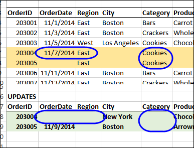
________________

Excel Roundup 20141110

One Excel annoyance is that after you select a group of cells, you can’t unselect one of them. For example, you might want to format specific cells, or create a named range, and you accidentally include a cell that shouldn’t be in the group. You can’t click on that cell to unselect it – you have to start over, and select more carefully the next time.

To solve that problem, Doug Glancy has created a free tool that you can download — SelecTracker.

Next, we need a version that lets you unselect one cell within an large area, e.g. if you drag down from A2:A7, click on cell A5, to unselect it.

Continue reading “Excel Roundup 20141110”

Excel Numbers Do Not Sort or Add Correctly

Last week, I heard from someone who was having a problem sorting some numbers in Excel. He sent me a small sample file that showed a few of the dates and numbers that just wouldn’t sort correctly.

My first guess was that the data had been copied from a website – that can cause some strange behaviour, when you paste it into Excel. A quick check with the COUNT and COUNTA functions showed that none of the values in cells C3:C6 were real numbers – they were text.

numbertext01

Continue reading “Excel Numbers Do Not Sort or Add Correctly”