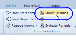
Last week, you saw my macro for adding worksheet data to the Excel footer, and formatting a date in the Excel footer. In that example, you had to run the macro by going to the View tab, and clicking the Macro command.
To make the process easier, I decided to add event code to the workbook, so the macro would run automatically.
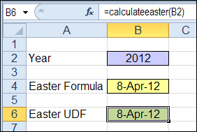
Easter has passed for this year, but it’s never too early to figure out when Easter will occur next year. Then, you can book your vacation for that date, and be out of town when the family shows up for Easter dinner!
It’s Fancy Footer Friday! Check with your boss – maybe you can leave early to celebrate.
This week, I’ve been working on Excel printed reports, and one of my clients wanted some fancy features in the footer. There are built-in footer options in Excel, but my client wanted to pull information from the worksheet, and format the date, so we needed some footer programming. Continue reading “Excel Footer with Formatted Date”
When you add comments to an Excel worksheet, they pop up to the top right of the cell, when you point to a cell with comments.
That’s fine most of the time, but if the cell is near the top or right of the window, you might not be able to read the comment.
Move Comments with Macro
Unfortunately, you can’t control the comment’s popup position, but with a bit of programming, you can show the comment in the centre of the screen, when you click on the cell.
Centre Excel Comments Code
Paste the following code onto a worksheet module. Then, when you click on a cell that contains a comment, that comment is shown in the centre of the active window’s visible range.
Private Sub Worksheet_SelectionChange(ByVal Target As Range)
 'www.contextures.com/xlcomments03.html
 Dim rng As Range
 Dim cTop As Long
 Dim cWidth As Long
 Dim cmt As Comment
 Dim sh As Shape
Application.DisplayCommentIndicator _
      = xlCommentIndicatorOnly
Set rng = ActiveWindow.VisibleRange
cTop = rng.Top + rng.Height / 2
cWidth = rng.Left + rng.Width / 2
If ActiveCell.Comment Is Nothing Then
  'do nothing
Else
   Set cmt = ActiveCell.Comment
   Set sh = cmt.Shape
   sh.Top = cTop - sh.Height / 2
   sh.Left = cWidth - sh.Width / 2
   cmt.Visible = True
End If
End Sub
More Excel Comment Macros
For more Excel comment macros, please visit the Excel Comment VBA page on the Contextures website.
______________
How do you calculate distance? In the small town where I grew up, distance was measured in blocks or travel time. For example, my school was about 5 blocks away (much further in the winter!) and my grandparents lived 5 minutes from our house – or 6 minutes during rush hour.
Longitude and Latitude
Sometimes you need more precise measurements, and Excel MVP, Jerry Latham, has an Excel user defined function that will help you. It’s designed to calculate accurate measurements, based on the longitude and latitude of your start and end points.
Why a user defined function? Unfortunately, an Excel worksheet formula isn’t accurate enough, if you need precise distances.
Jerry used to work in air traffic control, and he explains the problem with “almost” accurate worksheet formulas:
Typically they are short by some number of meters, typically about 20 to 30 feet per statute mile, and after flying just 30 or 40 miles, I wouldn’t care to land several hundred feet short of the approach end of a runway, much less be off by over 7 miles on a trip between Los Angeles and Honolulu.
Excel User Defined Function
On the Excel Latitude and Longitude Calculations page, Jerry outlines the problems with calculating distance in Excel, and describes his challenges in creating a solution.
You can read about Jerry’s journey to the final distance calculation solution, and copy Jerry’s Longitude and Latitude code to your own workbook.
Or, download Jerry’s sample file, and work with the code and worksheet examples there.
_____________
Last year, I showed that you could combine text in Excel by using the ampersand (&) operator, instead of the CONCATENATE function. That makes it much easier for those of us who are lazy, or can’t remember how to spell concatenate.
Last week someone sent me an Excel file that was having problems – it wouldn’t save properly, and there were a few other strange behaviours. The file had been working well for a few years, but recently started acting up.
The file was used in a factory, where the technicians filled in data, and printed the file, a few times each day. To print, they clicked a button on the data entry sheet. A macro printed the data entry sheet, copied the latest data to a storage sheet, and cleared the data entry cells.
Danger!
When I tried to open the file, Excel 2010 warned me that the file could be dangerous – not a good sign!
I ran the file through my virus scanner, and nothing malicious was found, so I opened the file in Excel 2003. No complaints from that version.
Excel Security Notice
What’s Hiding Under There?
When I switched to the storage sheet, there was some mysterious flickering, 2 buttons, and a partially covered button. I moved all 3 buttons, to see what was under them. Surprise! There were more buttons, and below those, more buttons.
With a bit of code, I did a quick count of the buttons on that worksheet. Debug.Print ActiveSheet.Shapes.Count
Under the 3 visible buttons, there were almost 7000 buttons. Yikes!
Every time the original data was copied and pasted onto this sheet, the 2 original buttons were being copied and pasted on top of the previous buttons. No wonder the workbook was having problems!
Fix the Problem
To clean up the storage sheet, I deleted all of the buttons, except one copy of each.
Then on the data entry sheet, I changed the button settings, so they don’t move or size with the cells.
Right-click on the button (these are buttons from the Form Control toolbox)
Click Format Control
On the Properties tab, select ‘Don’t Move or Size with Cells’, and click OK
Now, if the data entry sheet is copied and pasted, the buttons won’t be included.
If you’re copying and pasting cells, day after day, remember to check the settings for any buttons, or other shapes, that are on those cells. Don’t get buried under a mountain of buttons!
__________
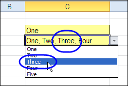
In Excel, you can use data validation to control (to some extent!) what users can enter in a cell. One option is to create a drop down list, so users can only select from a list of valid options.
There’s a popular sample file on my website, that lets you select multiple items from a data validation drop down list. Since the original article, I’ve posted updates:
Long ago, Dave Peterson created an Excel worksheet data entry form, so you could enter records on one sheet, and store the data on another sheet. Then, you can hide the data entry sheet, so users don’t accidentally change any of the old records.
There have been a few version of the data entry form file, including the the previous version, in which you could also update the selected record. This way, the data sheet can still be hidden, but users can make changes to the existing records.
Delete the Current Record
In a comment, Bryan asked for a Delete button too. In this new version, that feature is added. (Thanks, Bryan, for the suggestion!) Use this version if you really trust your workbook users – and keep good backup files!
When you click the Delete button, a message appears, asking you to confirm that you want to delete the record.
If you click No, the deletion is cancelled.
If you click Yes, the record is deleted from the database worksheet, and the data entry cells are cleared.
The file is in Excel 2003 format, and is zipped. After you unzip the file and open it, enable macros, so you can use the worksheet buttons.
_____________


 How do you calculate distance? In the small town where I grew up, distance was measured in blocks or travel time. For example, my school was about 5 blocks away (much further in the winter!) and my grandparents lived 5 minutes from our house – or 6 minutes during rush hour.