Excel REPT Function Examples Groundhog Day

Happy Groundhog Day! Have you made plans that you’ll be happy to repeat, day after day? Maybe these Excel REPT function examples will give you some ideas! There are written steps, screen shots, and 3 videos below.

REPT Function Minimum Row Height

First, if you’ve set up a nicely formatted named Excel Table, you can use the REPT function in one column, to set a minimum row height.

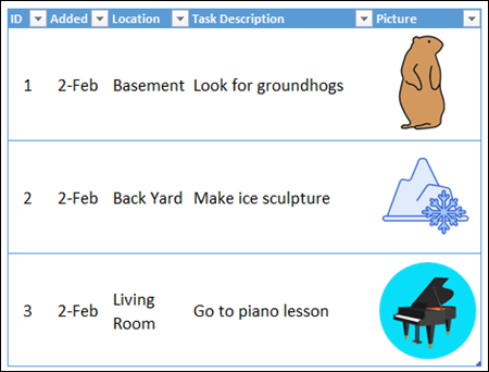
Here’s the formula in the Picture column, in the screen shot below, to make sure those cute pictures don’t get squished.

=REPT(CHAR(10),5)

In the formula, REPT repeats a line break character – CHAR(10) – 5 times, and that keeps all the rows the same minimum height.

Thanks to AlexJ, who suggested this technique for working with tables.

You can see more of AlexJ’s work on my Contextures site.

Make In-Cell Charts

Next, here’s another fun thing to do with the Excel REPT function – make little in-cell charts.

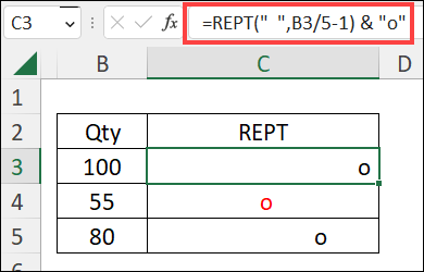
For example, here are the steps to make a set of simple dot plot charts, based on the numbers in column B.

In cells B3:B5, type 100, 55 and 80
In cell C3, type this formula:
- =REPT(” “,B3/5-1) & “o”
Copy the formula down to row 5
Adjust the width of column C, so the dot (“o”) is at the right edge in cell C3
After that, you can change any of the numbers in column B, and the related chart will also change

In this formula:

The REPT function repeats a space character (” “).
The number of repetitions is calculated from the number in column B, divided by 5, with 1 subtracted.
I divide by 5 to keep the bar charts shorter

At the end of the formula, a lower-case letter “o” is added to the REPT result.

Find Last Text Entry in Column

And here’s one more example – it combines REPT with VLOOKUP, to find the last text entry in a column.

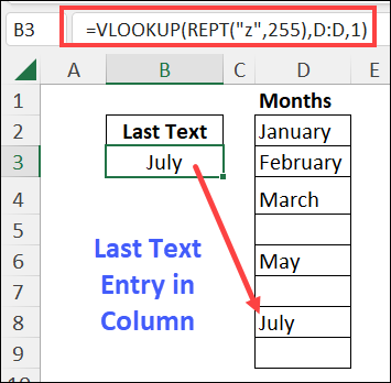
For example, with text items and blank cells in column D, use this formula to find the last text item:

=VLOOKUP(REPT(“z”,255),D:D,1)

In this formula:

The REPT function repeats the letter “z” 255 times
VLOOKUP searches for that text string, in column D.

Since it’s unlikely to find that text string anywhere in column D, VLOOKUP returns the last text entry that it found – July in this example.

Get Sample Files and More REPT Examples

See more REPT function examples on my Contextures site, and download the sample files there too.

Video: In-Cell Charts

This short video show other examples of in-cell charts with the REPT function.

The chart shows student grades, out of 100, in either a bar chart or dot plot.

Video: In-Cell Dot Plot for Stock Prices

Watch this short video to see how to set up an in-cell dot plot stock chart with the REPT function.

Video: Set Minimum Row Height

Watch this video to see the steps for setting minimum row height with the REPT function.

You can see the full written steps in this blog post.

_________________________