If you create a chart from worksheet data, and then filter the data, some of the chart date might disappear. Sometimes, that’s what you want — filter by Region, and see only the East’s sales in the chart. But, if you always want to see all the data in the chart, try this easy fix.
Note: There’s a similar problem with Excel’s in-cell Sparkline charts, and you can fix that too!
Watch the Show Hidden Data in Chart Video
This video shows how to change an Excel chart’s settings, so all the data will appear in the chart, even if some of the data rows or data columns are hidden.
There are written steps below the video.
Show Hidden Data in Excel Chart
Here’s how to fix a chart, so it isn’t affected if some data is hidden.
- Select the chart, and on the Excel Ribbon, click the Design tab
- Click Select Data
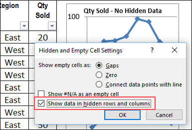
- Click the Hidden and Empty Cells button
- Add a check mark to ‘Show data in hidden rows and columns’
- Click OK, twice, to close the dialog boxes
After you change that chart setting, you can hide rows or columns in the worksheet data, and the chart data will stay visible
Test the Hidden Data Setting
To see the difference this option setting makes, test the feature in this embedded Excel file.
If you filter the Region column, one chart continues to show all the data, but the other chart has hidden data
Note: This embedded workbook might not work correctly in some browsers
___________________
Sparklines Problem for Hidden Data
Just like the normal charts in Excel, the in-cell Sparkline charts have a default setting that prevents hidden data from showing. Sparklines are available in Excel 2010 and later.
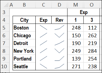
In this screen shot, column N is hidden on the worksheet. That column has the “Month 2” data for expenses.
- In column C, the Expense sparklines only have 2 data points.
- None of the Revenue data is hidden
- The Revenue sparklines, in column D, have 3 data points
Fix Sparklines to Show Hidden Data
To show the hidden data in your sparklines, follow these steps:
- Select the sparkline cell, or one group of sparkline cells
- NOTE: You can’t change multiple sparkline groups at the same time
- On the Excel Ribbon, click the Sparkline tab
- Click the Edit Data command
- Next, click the Hidden & Empty Cells command
- Add a check mark to the Show Data in Hidden Rows and Columns setting
- Click OK, to apply that setting.
Get Excel Workbooks and More Info
To get the sample workbooks for charts and sparklines, go to the Hidden Chart Data page on my Contextures website.
That page has more details showing hidden data, and there are macros there too, if you have to change the hidden data settings for lots of charts or sparklines.
Both of the sample files are zipped, and in xlsm format. The files contain the macros from the Hidden Chart Data page, so be sure to enable macros, if you want to test the code.
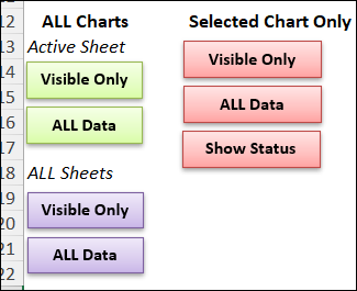
In the Hidden Chart Data workbook, there are worksheet buttons set up, so it’s easy for you to test the macros.
Related Info
Show Excel Sparklines for Hidden Data
___________________
Fix Excel Chart to Show Hidden Data from Worksheet
___________________


