
Instead of adding and removing pivot table values one at a time, click a Slicer, to quickly add and remove them, in groups. Most pivot tables won’t need this, but for source data with lots of numeric fields, this slicer technique can make things easier.
Slicer Demo
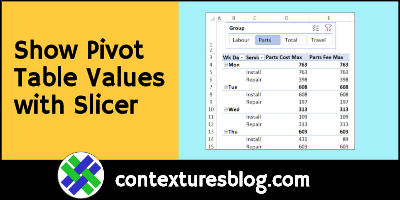
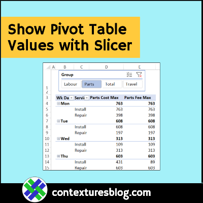
In this example, there’s a table with work order data, and a pivot table based on that data. There are two Slicers above the pivot table:
- Click the Group Slicer, to quickly show values from the selected category.
- Click the Function slicer to set the function and heading for each value

Source Data Number Fields
This pivot table is based on a table with work order records, and about half of the columns have numbers. Those number columns fall into four categories (groups).
- Travel — Kms, Km Fee
- Labour — Lbr Hrs, Lbr Cost, Lbr Fee
- Parts — Parts Cost, Parts Fee
- Total — Total Cost, Total Fee
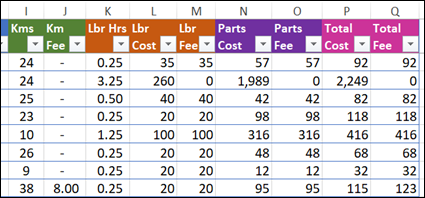
In the sample file, I colour coded the column headings, just to make the groups easier to identify.
- headings don’t need to be coloured
- columns could be in any order in the source data
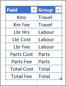
Value Groups List
To put the fields into groups, all the numeric fields are listed in an Excel table. In the table’s second column, each field is assigned to one of the 4 value groups.
If you’re setting this up in a different workbook, you can create as many groups as your data needs, and fields can be assigned to multiple groups, if needed.
For example, all the Labour and Parts fields could be listed again, in a group named Parts & Labour.
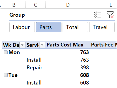
Pivot Table and Slicer
A pivot table was built from the Value/Group table, and it has the Group field in its Filter area.
There’s a Slicer connected to that pivot table, and that’s what you click to select one of the Value groups, to show in the main pivot table.
Run a Macro
When you click the Slicer, it updates the connected pivot table, and a macro runs automatically, to:
- remove all the current value fields
- add all fields from the selected group
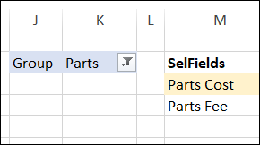
A dynamic array formula creates a list of all the selected group’s fields:
- =SORT(FILTER(tblFields[Field], tblFields[Group]=K3))
The formula is in cell M4, and it spills into the cells below.
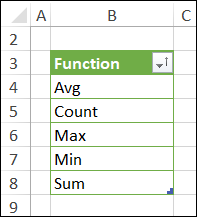
Function Slicer
There’s a function slicer in the workbook too, where you can select from 5 common summary functions.
It’s set up in a similar way, with a list of functions, a pivot table based on the list, and a Slicer connected to the pivot table.
Get Details & Sample File
To get the sample file, and to see the details on how this technique works, go to the Value Group Slicers page on my Contextures site.
The file is zipped, and is in xlsm format. The file contains macros which run when the slicers are clicked. Be sure to enable macros when you open the workbook, if you want to test the Slicers.
_________________________
Show Pivot Table Values with Slicer
_________________________