Colour Bands in Excel Table Based on Dates

When you create a named table in Excel, you can colour the alternating rows with one of the built-in Table Styles. But how could you colour alternating groups of information, such as dates? This example shows show to create colour bands, based on dates, so it’s easy to see where each day’s data begins and ends.

Colour Bands in Excel

In the steps shown below, you’ll see how to use Excel conditional formatting to create colour bands, based on the data in one column..

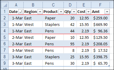
In this example, the sales rows for the dates are in alternating colours – blue and no fill. This technique was adapted from Chip Pearson’s site.

Add a New Column

First, we need to add a new column to the table, where a formula will check the date, and compare it with the date in the previous row.

In cell D1, type a heading for a new column – TRUE
In cell D2, enter this formula, to compare the dates:
=IF(A1=A2,D1,NOT(D1))
Press Enter, and the formula automatically fills down to the end of the table, with a result of TRUE or FALSE in each row.

How the Formula Works

The formula in cell D2 compares the date in column A, to the date in the cell above that

=IF(A1=A2,D1,NOT(D1))

If the dates are the same, the result is the value from column D, in the previous row

=IF(A1=A2,D1,NOT(D1))

If the dates are different, the result is the opposite of the value in the row above, because the Excel NOT function reverses TRUE and FALSE.

=IF(A1=A2,D1,NOT(D1))

In cell D2, the result is FALSE (the opposite of the TRUE in cell D1), because the date in cell A1 is not equal to the “Date” heading in cell A1.

NOTE: You could use either TRUE or FALSE as the heading in column D

Table Style Optons

Before you add the conditional formatting, turn off banded rows in your Excel table, if that feature is active.

Select a cell in the table
On the Excel Ribbon, click the Table Design tab
In the Table Style Options group, remove the check mark for Banded Rows.

Add Conditional Formatting

Then, follow these steps to add the conditional formatting that creates colour bands:

Starting from row 2, select all the data cells in the table
On the Home tab, click Conditional Formatting, New Rule
Click on “Use a formula to determine which cells to format”
In the formula box, type this formula, referring to the active data cell:
=$D2=TRUE
Click the Format button, and choose a fill colour for the rows that have TRUE in column D
Click OK, twice, to apply the formatting
(Optional) Hide the TRUE/FALSE column, to tidy up the worksheet.

Absolute Reference

In the conditional formatting rule, =$D2=TRUE, we use an absolute reference to column D ($D), instead of a relative reference (D).

With an absolute reference, all the columns will refer to the value in column D
With a relative reference, the formula would adjust in each column, and each cell would check its own value, instead of the cell in column D.

For example, the conditional formatting in column B would look for TRUE in column E, instead of column D. Column E is empty, so there’s no colour applied in column B.

Add a Border to Separate Groups

Another way to separate the groups is with a top border, like I did with this list of dates.

You don’t been an extra column for this technique.

Colour Row Based on One Cell’s Value

This video shows how to format multiple cells in a row, based on on cell’s value, using an absolute reference.

Video Transcript:

With Excel’s conditional formatting, you can easily highlight a cell if it’s over or under a certain value, or if it meets a value that you’ve set.

But in some cases, instead of just a single cell, you might like to highlight a whole row in a table, if one of the cells in that row is over a certain number or under.

In this case, we would like to highlight each row in this list if the number of units sold is greater than 75.

So to do that, I’m going to select all of the rows, all of the columns in each row. So I’ve selected from A2 down to D10.

On the Ribbon, on the Home tab, I’ll click Conditional Formatting, and none of these preset rules will do exactly what I want. So I’m going down to New Rule, and in here I’ll select a formula.

So I’m going to use a formula to determine how to color each row.

When I click that, there’s a spot where I can put the formula.

I want to, in each row, look at the value that’s in column B. So I’ll type =

And we want, from every column, we want to look at column B. So we have to lock that cell. We don’t want it to be relative, we want it to be absolute.

So type a $ to lock that in. And then B.

And we want, in this case, the active cell we can see is white, where the other cells are highlighted with blue.

We can see that, in the name box, A2 is showing up. So that’s the active cell, so the active row is 2. So I’m going to type 2 here.

We’re going to check what’s in B2 and see if it’s greater than 75. So that’s our test.

And if it is greater than 75, we want to format it. So I’ll click Format and I’ll choose a fill color, maybe a blue color and click OK, and click OK again.

And now, any row where the number of units is greater than 75, all four cells in that row are colored blue.

More Conditional Formatting Examples

See more conditional formatting examples on my Contextures website, and download the sample file there.

_________________