Count Duplicate Number Sets in Excel

Recently, someone asked me how to count duplicate number sets. There were hundreds of rows, with 6 numbers in each row. Did any of the number sets appear in the list more than once? How would you solve this problem, and count duplicate number sets?

Count Duplicate Number Sets

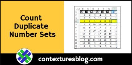
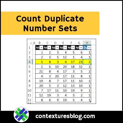
To find a solution, I set up a small table with random numbers. There are 11 rows of numbers, and 6 columns.  The 7th column, Dups, is where I tested my formulas.

How Many Matches?

In each row, the goal is to find out how many times that set of 6 numbers appeared in the table.

It doesn’t matter if the numbers are in a different order. For example — 1,2,3,4,5,6 is be a duplicate of 3,4,5,1,2,3 — all 6 numbers are the same.

How would you calculate the number of matches?

Get the Sample Data

There are solutions below, but before you look at them, try to find your own solution.

Download the sample file (#4) from the Excel Count Functions page on my Contextures site.

The sample data is in a table on the Challenge sheet.

Solution 1: It’s Complicated

I’ll confess to doing a Google search when this question arrived in my email. There were suggestions for macros and User-Defined Functions, but I didn’t try those.

Finally, I found an array-entered formula on StackOverflow, which pointed me in the right direction. Here’s the formula, which was for a list with 4 columns and 1000 rows:

=IF(SUM(IF(MMULT({1,1,1,1}, TRANSPOSE(COUNTIF($A1:$D1, $A$1:$D$1000)))=4,1))>1, “duplicate”, “unique”)

That certainly looked complicated!

Adjusting the Formula

I needed to adjust the formula, so it would work with 6 columns, instead of 4.

• MMULT({1,1,1,1,1,1}
• COUNTIF(B2:G2

My list has 11 rows, instead of 1000. (My data is in a named Excel table, so the range will adjust automatically if the table size changes.)

• $B$2:$G$12

And I wanted the number of duplicates, not text, so the first IF was removed. Here’s my revised formula (array entered, with Ctrl+Shift+Enter):

=SUM(IF(MMULT({1,1,1,1,1,1},TRANSPOSE(COUNTIF(B2:G2,$B$2:$G$12)))=6,1))

How It Works

Here’s a brief explanation of how the works. There are more notes in the sample file, on the Solution01 sheet.

1. COUNTIF checks each table row, to see if each number has a match in the formula’s row. The result is an array with 11 rows and 6 columns
2. MMULT will return an array with the number of matches in each row. We need that array to have 1 row, and 11 columns (1 column for each set of numbers)
   1. Array1 is {1,1,1,1,1,1}
   2. For Array2, TRANSPOSE switches the rows and columns in the COUNTIF array, to create an array with 6 rows and 11 columns.
3. IF returns a 1, if the number of matches is 6 (all others = FALSE)
4. SUM adds up all the 1s to give the number of duplicate sets

Worksheet Results

The screen shot below shows what the COUNTIF calculations would look like for Row 4, with the rows and columns transposed.

The MMULT result is 1 row, with 11 columns, and the final SUM is 2, because rows 4 and 6 have the same set of numbers.

Slow Calculations

This formula isn’t too bad in a small set of numbers, but could take a long time in a larger dataset.

In the sample file, there’s a sheet named LargeSet, which has 1500 number sets, if you want to test that.

Solution 2: Power Query

The second solution in the sample file is from Jonathan Cooper, who used Power Query (Get & Transform).

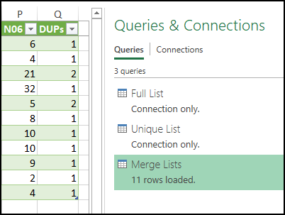
• Full List has all the rows, an index column, and a column with sorted numbers
• Unique List only has the Index column and sorted numbers, with duplicates removed
• Merge List combines the Full and Unique lists, and calculates the count for each unique number set

Solution 3: SMALL and TEXTJOIN

Jonathan’s solution had a comma-separated list of sorted numbers in one step. That led me to a different Excel formula solution, using the SMALL and TEXTJOIN functions.

To show how it works, the SMALL results are done in 6 separate columns. Here’s the formula in cell I4:

=SMALL($B4:$G4,I$3)

TEXTJOIN combines the results. Here’s the formula in cell O4:

=TEXTJOIN(“|”,,I4:N4)

And COUNTIF returns the number of instances of the comma-separated list from column O:

=COUNTIF([Sorted],[@Sorted])

All-In-One Sorted List

Instead of using helper columns for the SMALL function, you can use an array-entered formula to get the same results.

Put this formula in cell O4 (array-entered):

=TEXTJOIN(“|”,, SMALL(B4:G4, ROW($1:$6)))

Then, delete the columns with the SMALL formulas.

Count Duplicate Number Sets Sample File

To find your own solution, and to see the other solutions, download the sample file, named Count Duplicate Number Sets, from the Excel Count Functions page on my Contextures site.

The sample data is in a table on the Challenge sheet, and there is a larger dataset on the sheet name LargeSet.

NOTE: The workbook does not contain macros, but you will see an alert about a data connection, because of the Power Query solution.

__________________

Count Duplicate Number Sets

__________________