
At work, we use Excel for serious projects, like financial reports or marketing forecasts. Excel is useful at home too, for personal tasks. I keep daily notes, and I added conditional formatting for weather data, to make the columns easier to read.
Weather Data With Formatting
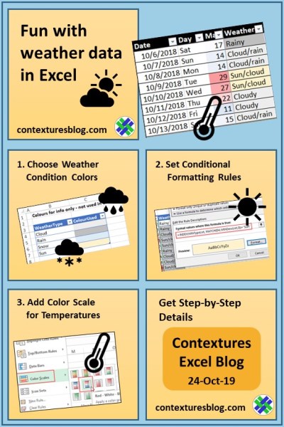
Here’s a screen shot of my conditional formatting for weather data. It’s easy to see the warmer and cooler days, and what the sky was like each day.
I wanted to see what last October was like, and we had a couple of hot sunny days back then!

Get the Weather
I get the daily temperature and weather conditions from the Government of Canada Weather page. Click any city, province or territory on that map, to see the current conditions and the forecast.

Near the top of the City page, there’s a forecast, with the maximum temperature and weather conditions.

At the bottom of the page, you can find the actual maximum from the previous day. That’s the number that I store in my weather log, along with my own description of the conditions.

If you’re a real weather nerd, there’s daily or historical data to download too. We won’t go down that rabbit hole though! Well, not today.
Weather Conditions
Besides the weather log sheet, there’s another sheet in my Excel file – Admin_Lists. That sheet has two named Excel tables – one for weather types, and one for weather descriptions.
The weather types table is named tblWType, and it has 2 columns.
- Types are listed in the first column
- Colours are shown in the second column. These are for info only. We can’t use them in the conditional formatting rules, unfortunately.

The weather descriptions table is named tblWeather, and it also has two columns.
- The weather descriptions that I use are in the first column.
- A weather type for each description is selected in the second column.

Named Ranges
There are also 3 named ranges on the Admin_Lists sheet:
- WthTypeMain – Items in the Wtype column, in the Weather Types table
- WthDescList – Items in the WthDesc column, in the Weather Descriptions table
- WthTypeList – Items in the WthType column, in the Weather Descriptions table

Weather Type Drop Down
In the WthType column, in the Weather Descriptions table, there are drop down lists, created with data validation.
The list is based on the named range – WthTypeMain.

Weather Log Sheet
On the WeatherLog sheet, there’s one named table – tblWthLog.
- Date is typed in column 1
- A TEXT formula shows the day name in column 2: =TEXT(A4,”ddd”)
- Maximum temperature is typed in column 3
- Weather description is selected in column 4
- The weather drop down is based on the named range – WthDescList

Temperature Conditional Formatting
In the Temp column, I used colour scale conditional formatting. Here’s how to set that up:
- In the Weather Log table, click at the top of the Temp column heading, to select all the temperatures (not the heading)
- On the Excel Ribbon’s Home tab, click Conditional Formatting
- Point to Color Scales
- Click on the Red-White-Blue color scale

There’s a video at the end of this post, that shows another example of using a color scale for temperatures.
Check the Color Scale Results
After you apply the conditional formatting color scale, scroll through the weather log, to see the results.
Instead of trying to read a long list of numbers, you can just check for dark red or dark blue cells, to find the highs and lows in the Temp column.

Weather Conditional Formatting Rules
It takes a bit more work to set up the conditional formatting rules for the Weather column.
There are 4 weather types – Sun, Cloud, Rain, and Snow – and we’ll need a separate rule for each of those types.
In the rule, we’ll use an INDEX/MATCH formula, to find the weather type for each description.
We’ll test the formula on the worksheet first, before creating the conditional formatting rule.
Type this formula in cell F4 on the WorksheetLog sheet:
=INDEX(WthTypeList, MATCH(D4, WthDescList,0))
Then, drag the formula down a few rows, to see the results. It finds the weather type for each description in column D.

Leave the formula in column F for a few minutes, while you create the conditional formatting rules. You can clear those cells later.
Set Up the Rules
Follow these steps to set up the first rule, for Sun:
- On the worksheet, copy the INDEX/MATCH formula from cell F4
- In the Weather Log table, click at the top of the Weather column heading, to
select all the description cells (not the heading) - NOTE: Cell D4 will be the active cell – you can see its address in the Name Box, to the left of the Formula Bar
- On the Excel Ribbon’s Home tab, click Conditional Formatting, then click New Rule
- Under “Select a Rule Type”, click on “Use a formula to determine which cells to format”
- Click in the Formula box, and press Ctr+V to paste in the INDEX/MATCH formula
- Click at the end of the formula, and type: =”Sun”
- Click the Format button, and click the Fill tab
- Click the fill colour that you want for sunny days
- Click OK, twice, to apply the conditional formatting
In the Weather column, the Sun/cloud days show the colour that you selected. Those rows also show “Sun” in the temporary formulas in column F.

Create 3 More Rules
Next, follow the same steps, to create 3 more rules, for the other weather types:
Cloud (light grey)
- =INDEX(WthTypeList, MATCH(D4,WthDescList,0))=”Cloud”
Rain (dark grey)
- =INDEX(WthTypeList, MATCH(D4,WthDescList,0))=”Rain”
Snow (light blue)
- =INDEX(WthTypeList, MATCH(D4,WthDescList,0))=”Snow”
The Weather column should show the colours that you selected for each weather type.
For example, here’s the delightful weather that we had last February. We were certainly glad to see a bit of sun on February 23rd!

You can clear the temporary formulas from column F now. They were just there as “helpers” while creating and checking the rules.
See All the Rules
To see all the rules that you’ve set up, follow these steps:
- On the Excel Ribbon’s Home tab, click Conditional Formatting, then click Manage Rules
- At the top of the Conditional Formatting Rules Manager, select “This Worksheet”
The Rules Manager shows a list of the rules set for the active sheet.
- The Graded Color Scale rule is in the list, and applies to cells in column C.
- The INDEX/MATCH formula rules are listed too, and they apply to cells in column D.

TIP: To see the full formula for a rule, point to it in the list of rules. A popup appears, to show the full rule.

Get the Sample File
To get the completed sample file with the conditional formatting for Weather Data, go to the Conditional Formatting Examples page on my Contextures site.
The zipped file is in xlsx format, and does not contain any macros.
Video: Temperature Color Scale
This video shows another example of using a conditional formatting color scale to highlight low and high temperatures.
See the setup details for this example.
_____________
Conditional Formatting for Weather Data


______________