In a perfect world, nobody would ever make a mistake in Excel. Every formula would be flawless, and every bit of data would be valid. Unfortunately, that’s not the case. When mistakes happen, there are built-in errors, like #N/A, but why not create your own Excel formula error values, and show those too?
Excel Error Values
I’m sure you’re familiar with most of the built-in Excel formula error values. Microsoft calls them hash errors, because of the character at the beginning.
- #NUM!
- #VALUE!
- #N/A
- #DIV/0!
- #REF!
- #NAME?
- #NULL!
Most of the hash errors end with an exclamation mark, but #NAME has a question mark, and poor old #N/A doesn’t get any punctuation. So sad.
Correcting Formula Errors
You can find troubleshooting tips for all the error values on the Microsoft site. Here’s a brief note on each hash error, and a link to the related Microsoft help page
#NUM! – Numeric values aren’t valid, or an iteration function can’t find a result, or the formula result is a number that’s too large or small to be shown. #NUM! Help
#VALUE! – Something is wrong with the formula or the cells that it references, or it could be something else, who knows? Microsoft admits that this one is vague, but has some common fixes #VALUE! Help
#N/A – The formula can’t find the thing it was asked to look for, usually with VLOOKUP, MATCH, etc. #N/A Help
#DIV/0! – The divisor is a zero, and Excel can’t divide by zero. #DIV/0! Help
#REF! – The formula refers to a cell that isn’t valid. Perhaps a column or row is deleted, or a VLOOKUP range has 3 columns, and you ask for a result from column 4. #REF! Help
#NAME? – Usually caused by a type in a function name or a defined name. Or, you put text into a formula, but didn’t enclose it with double quote marks #NAME? Help
#NULL! – The formula refers to a range that doesn’t exist. Often caused by the intersection operator (the space character) #NULL! Help
Create Your Own Hash Errors
Instead of using Excel’s built-in hash errors, it might be fun (and helpful) to create your own hash errors. Thanks to UniMord for this suggestion!
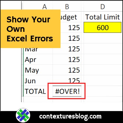
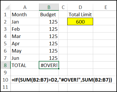
Here’s one example – a 6 month budget, with a limit of 600. In the total cell, an IF function checks the sum, and if it’s over the limit, a custom hash error appears – #OVER!
=IF(SUM(B2:B7)>D2, “#OVER!”, SUM(B2:B7))
It looks like an official warning from Excel, so perhaps your co-workers will pay attention to it!
Warning: Use this technique with discretion, because your co-workers might not like it! Be sure to add notes to the workbook, or cell comments, explaining what your custom hash errors mean.
Use a Custom Number Format
Another way to show a custom hash error is with conditional formatting.
In this example, there is a conditional formatting rule on the Total cell (B8)
=B8>D2
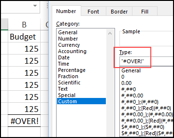
If that condition is met, the cell shows a custom number format:
“#OVER!”
Get the Sample File
I’m sure that you can think of other hash errors to show in your workbooks! What suitable-for-work errors would you add to your Excel files?
To see the custom hash errors from this blog post, go to the Excel Sample Files page on my Contextures site.
In the Functions section, look for FN0060 – Create Custom Hash Errors in Excel.
The zipped file is in xlsx format, and does not contain any macros.
________________________
Show Your Own Excel Formula Error Values
________________________


While this is cool and fine for hobby projects, I believe showing custom error values has more disadvantages than benefits, especially if you do it with custom number formatting.
My gripe is that the error message is non-transparent to the user. If there’s a formula, they can audit it, but custom formatting takes some digging to understand. The user needs to understand the error and what caused it. I prefer inserting meaningful error messages with nice bright bold red font (using conditional formatting) to notify of some broken rule, such as going overbudget, for example. This is especially true if the end user is not an Excel expert and might get frustrated with a weird error code. They might even go online to ask people what that error means.
Thanks, Vit, and I’ve added a warning in the blog post.
Hi all
Thanks Debra for your amazing work here.
This is about another blog entry, more or less called :
Excel Form Control Buttons
(There is no room for comments there) (this is why I comment here)
A code snippet is nicely provided under the paragraph titled :
List All Buttons, How to Use This Macro
In my case the code was not able to list all my buttons because my 2 buttons were
Button 1
Button 13
and after trying Button 2 the code went into the exit for instruction.
I don’t especially want you to publish this comment, the reason I make it is just to help improve in case you think It can be of some use. So feel free to erase this comment or not publish it.
Therefore I slightly changed the code like this :
(see comments in the code that underline my changes)
Sub ListAllButtons()
Dim wsList As Worksheet
Dim wsA As Worksheet
Dim btn As Button
Dim sh As Shape
Dim BtnList As ListObject
Dim lRow As Long
Dim lBtns As Long
Dim lNum As Long
Dim lMax As Long
Dim lCount As Long
Dim LastCol As Long
Dim strBtn As String
Set wsA = ActiveSheet
Set wsList = Sheets.Add
lRow = 1
LastCol = 7
lMax = 100000
lBtns = wsA.Buttons.Count
On Error Resume Next
With wsList
.Range(.Cells(lRow, 1), _
.Cells(lRow, LastCol)).Value _
= Array(“Internal Name”, “Display Name”, _
“Index”, “ID”, “Row”, “Col”, “Caption”)
lRow = lRow + 1
For lNum = 1 To lMax
Set btn = Nothing
‘ lCount = lCount + 1
If lCount = lBtns Then Exit For
strBtn = “Button ” & lNum
Set btn = wsA.Buttons(strBtn)
‘OPTIONAL – make display name
‘ same as numbered default name
‘ this might help if multiple buttons have
‘ the same display names
‘btn.Name = strBtn
If Not btn Is Nothing Then
‘added by jd start
lCount = lCount + 1 ‘ in fact that instruction was moved from the line I commented 14 lines above
‘If lCount = 2 Then btn.Caption = “Clear A3” ‘ Optional : to show a specific text on your button.
‘added by jd end
Set sh = wsA.Shapes(btn.Name)
.Range(.Cells(lRow, 1), _
.Cells(lRow, LastCol)).Value _
= Array(strBtn, sh.Name, btn.Index, _
sh.ID, sh.TopLeftCell.Row, _
sh.TopLeftCell.Column, btn.Caption)
lRow = lRow + 1
End If
Next lNum
Set BtnList = .ListObjects.Add(xlSrcRange, .Range(“A1”).CurrentRegion, , xlYes)
BtnList.TableStyle = “TableStyleLight8”
BtnList.HeaderRowRange.Columns.AutoFit
BtnList.DataBodyRange.Columns(1).AutoFit
End With
End Sub
There’s no reason to hide the reason:
“#OVER! ” & $D$2
Great idea, thanks!
The text within your post states 6,000 (six thousand) whereas the image is showing 600 (six hundred).
Thanks, and I’ve fixed the text to say 600