With Excel’s conditional formatting options, you can highlight cells based on their values, or add colour scales, icons and data bars to the cells. There are built-in rules to highlight top or bottom values, and you can also create your own rules, as shown below.
Top/Bottom Formatting
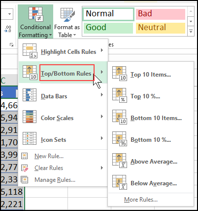
To see Excel’s conditional formatting options to highlight top or bottom values, click the Conditional Formatting command on the Ribbon’s Home tab.
Then, point to the Top/Bottom option, to see all the available variations.
Top/Bottom Limitations
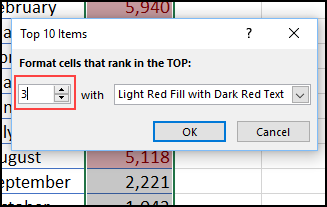
Those built-in rules are handy, but you have to type your top and bottom settings in the setup window. You can’t refer to a worksheet cell, to make the rule flexible.
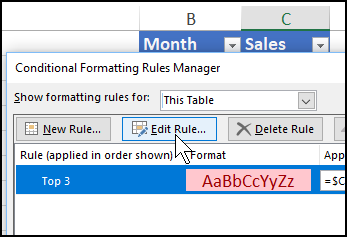
Later, if you want to highlight the top 4 values, you would have to go into the Conditional Formatting rule manager, and change the number there.
Highlight Top or Bottom Values
Instead of using the built-in conditional formatting rules to highlight top or bottom values, see how to create your own.
The video below shows two examples:
- Top 3 values in a list
- Bottom X values in a list
The first example uses a typed number, then the second example shows how to make the rule flexible. There are written instructions below the video.
To download the sample workbook, go to the Conditional Formatting Examples page on my Contextures website.
Top 3 Values
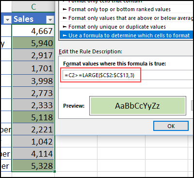
In the video’s first example, the 3 highest numbers in the list of monthly sales will be highlighted.
Our conditional formatting rule uses Excel’s LARGE function, which has 2 arguments:
- numbers to check — $C$2:$C$13
- the nth highest number to return — 3
The rule compares each number to that 3rd highest number.
- C2>=LARGE($C$2:$C$13,3)
Follow these steps to apply the conditional formatting:
- Select the numbers in the Sales column (C2:C13)
- On the Ribbon’s Home tab, click Conditional Formatting, then click
New Rule - Click Use a Formula to Determine Which Cells to Format
- In the formula box, enter the LARGE formula,
=C2>=LARGE($C$2:$C$13,3) - Click the Format button.
- Select formatting options (light green fill),
click OK - Click OK
Bottom X Values
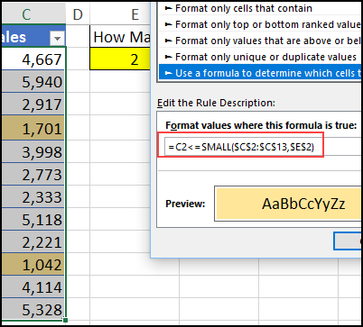
In the video’s second example, the lowest numbers in the list will be highlighted.
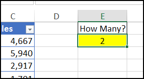
This time, the conditional formatting formula will refer to a worksheet cell (E2), to create a flexible rule.
This formula uses the SMALL function, which is similar to LARGE, but returns the nth smallest number.
Follow these steps to apply the conditional formatting:
- Select the numbers in the Sales column (C2:C13)
- On the Ribbon’s Home tab, click Conditional Formatting, then click
New Rule - Click Use a Formula to Determine Which Cells to Format
- In the formula box, enter the SMALL formula,
=C2<=SMALL($C$2:$C$13,$E$2) - Click the Format button.
- Select formatting options (light orange fill),
click OK - Click OK
Test the Flexible Rule
To test the flexible conditional formatting rule:
- Type a different number in cell E2, to change the number of cells that are highlighted
- Delete the number in cell E2, or type a zero, so that none of the numbers are highlighted
Download the Workbook
To download the sample workbook, go to the Conditional Formatting Examples page on my Contextures website.
The zipped file is in xlsx format, and does not contain any macros.
______________________
Highlight Top or Bottom Values in Excel List
______________________



How to highlight two large value row wise in excel.
In a student Marksheet of 200 students, each students top 2 marks must be considered to highlight these each top 2 students marks it will be tedious job.
Kindly help me with formula for the consolidated sheets
=C14>=LARGE(C$14:C$22,2)
How can I highlight the cells (from lowest value) which the sum of these cells are below 20% of the whole range?
For example, there is an array of 10 values, from 1 to 10. I want to highlight those cells which contribute 20% of the overall total. Then I expect the system returns with cells containing value of 1, 2, 3 and 4 to be highlighted.
Thanks a lot!