To use VLOOKUP, the value you’re looking for has to be in the first column of the lookup range. But what if your lookup table has Scores in column 3, and you need a description from column 2? Here’s how you can do an Excel VLOOKUP to the left.
Lookup Table
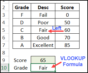
In the lookup table below, there are 3 columns, with letter grades, descriptions, and numeric scores.
A score is entered in cell C9, and we want our VLOOKUP formula to get the description from column C, using an approximate match for a Score.
Get Help from CHOOSE
To get the VLOOKUP to work, we’ll combine it with the CHOOSE function.
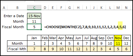
Usually, CHOOSE makes a simple selection from a list of options, such as finding the Fiscal Month, based on calendar month number.
For example, if the fiscal year starts in July (month 7), the fiscal months for January to December are in this order: 7,8,9,10,11,12,1,2,3,4,5,6
If we put that list of values in a CHOOSE formula, we can find the fiscal month number for the date in cell C6.
=CHOOSE(MONTH(C6), 7,8,9,10,11,12,1,2,3,4,5,6)
First, the MONTH function gets the month number (n) for the date, and the CHOOSE function returns the nth item in the list.
Today’s month number is 11 (November), and the 11th item in the list is 5.
NOTE: The month number in cell C3 is just for demo – it isn’t referenced in the CHOOSE formula.
CHOOSE Special Powers
Beyond making a single selection from a list, CHOOSE has special powers – it can create arrays too.
For our VLOOKUP, we’ll use CHOOSE to create a table array, with scores in the first column and descriptions in the second column.
The CHOOSE function will be added as the Table_Array argument for the VLOOKUP function.
=VLOOKUP(C9, Table_Array, 2, TRUE)
CHOOSE Table Array
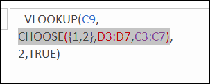
To create the table array in the VLOOKUP formula, add this CHOOSE formula:
=VLOOKUP(C9,CHOOSE({1,2},D3:D7,C3:C7),2,TRUE)
Instead of a single index number, CHOOSE has 2 numbers, inside curly brackets.
Those numbers inside the curly brackets – {1,2} – tell Excel to create a 2-column array, with Scores in column 1, and Descriptions in column 2.
CHOOSE rearranges the columns, putting the in the order that VLOOKUP needs, so you don’t need to physically change the table layout.
See the CHOOSE Array
To see the array that CHOOSE creates:
- Select the cell with the VLOOKUP formula
- Select the entire CHOOSE function in the formula bar
- On your keyboard, press the F9 key, to evaluate the selected part of the formula.
- Each pair of scores/descriptions is evaluated.

IMPORTANT: When you’re finished, press the Esc key, to exit the formula, without saving the changes.
VLOOKUP Gets the Description
The rest of the formula is just a basic VLOOKUP.
=VLOOKUP(C9, Table Array, 2, TRUE)
For the score entered in cell C9, VLOOKUP returns the value from column 2 of the table array, using an approximate match (TRUE).
Get the Sample File
Go to my Contextures site to download the sample file, and to see more examples for the CHOOSE Function.
The zipped file is in xlsx format, and does not contain macros.
______________________


I use EDATE () to convert to fiscal month, instead of CHOOSE ().
Hi
My Name is DPK and i have a probblem
i got a result like {0;1;0;0;0;0;0;3;4;6;0;0;0} in single cell and i want extract only number greater than {0} and i want result like {1;3;4;6;} or {1};{3};{4};{6} in single cell
do help in this matter