
If you’re planning a vacation trip, Excel can help. It’s a great place to keep your packing lists, and you can track your vacation spending too (if you really want to know the total!). I’ve just uploaded a new sample file that will show how far you’ll travel. Select cities, and formulas do a mileage lookup, with total distance from start to end.
Two City Mileage Lookup
The new workbook is based on a previous one, which showed the distance between two cities. Select a city name in each green cell, and see the distance between those two cities, in miles.
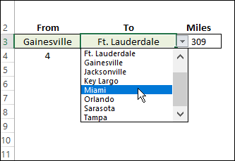
The distances come from a lookup table, shown below. Find the intersection of the two selected city names, and that is the distance between them.
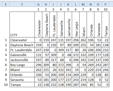
The data in that table is from the Florida Dept. of Transportation.
Plan a Vacation Trip
The old workbook was handy if you were going from one city to another, and then straight back home. But what about a longer journey, with stops at multiple cities?
Maybe you’d like to plan a trip to a few vacation spots in Florida, and see how far you’ll travel. I’ve put arrows on a Florida map, to show our imaginary vacation route. The trip starts from Gainesville, gets down to Sarasota, and then back home.
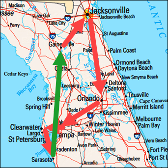
NOTE: I found a copyright-free map on The National Map site, which is run by the U.S. Geological Survey. Do not visit that site if you are easily distracted – there are lots of fascinating data collections and maps there. You have been warned!
Total Distance for a Vacation Trip
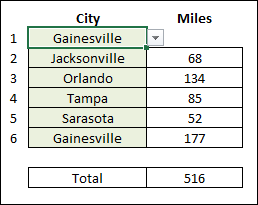
In the new workbook, there are data validation drop down lists where you can choose up to 6 cities.
There are formulas in the next column, to do a lookup from the mileage table, and another formula shows a grand total.
The Lookup Formula
To do the mileage lookup, the “Miles” column has an INDEX/MATCH/MATCH formula in each row. Read more about INDEX and MATCH on my website.
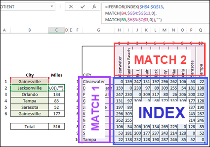
Here is the formula in cell C5:
=IFERROR(INDEX($H$4:$Q$13,
MATCH(B4,$G$4:$G$13,0),
MATCH(B5,$H$3:$Q$3,0)),””)
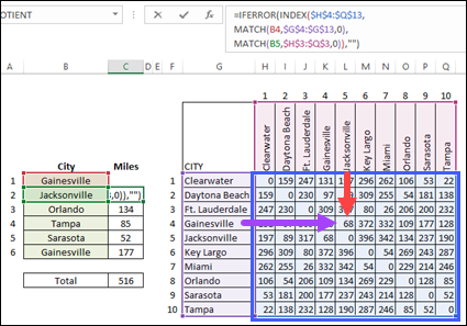
- The INDEX function returns a value from H4:Q13 (outlined in blue)
- The first MATCH function returns the row of the first city (in B4), from the vertical list of cities in G4:G13 (purple)
- The second MATCH function returns the column of the second city (in B5), from the horizontal list of cities in H3:Q3 (red)
NOTE: The IFERROR function puts an empty string in the Miles cell, if it can’t calculate the distance.
The distance from Gainesville to Jacksonville is 68 miles.
Get the Total Distance
The lookup formula from cell C5 is copied down to C9, to calculate the distance for each leg of the trip.
Then, in cell C11, there is a SUM function, to calculate the total miles for the trip.
=SUM(C5:C9)
Get the Mileage Lookup Workbook
To get the Mileage Lookup with Total Distance workbook, go to the Excel Sample Files page on my Contextures site. In the Functions section, look for FN0055 -Total Travel Distance Mileage Chart
The zipped file is in xlsx format, and does not contain macros.
________________

Comments are open for 60 days, on new posts, and closed for older posts.
I need help with how to create the exact formula scenario you provided for conditional formatting (highlighting) in the Match/Index portion of your tutorial. I went to the instructed zip file but you had gone in a completely different direction and instead it was a tutorial for high/low functionality. I work for a bank and I am building a table that uses drop downs to give us exact mileage between branches for travel expense purposes. I want to add the highlight feature but am having trouble figuring out how to formulate that based on example provided.