
Aside from staring at them closely, how can you compare two cells in Excel? Here are a few functions and formulas that check the contents of two cells, to see if they are the same.
Easy Way to Compare Two Cells
To compare the two cells, we’ll start with a simple check, then try more complex comparisons.
- Tip: You can see more ways to compare two cells on my Contextures site. Get an Excel workbook with all the examples from that page too.
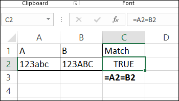
The quickest way to compare two cells is with a formula that uses the equal sign.
- =A2=B2
If the cell contents are the same, the result is TRUE. (Upper and lower case versions of the same letter are treated as equal).
Compare Two Cells Exactly
If you need to compare two cells for contents and upper/lower case, use the EXACT function. This video shows a few EXACT examples.
As its name indicate, the EXACT function can check for an exact match between text strings, including upper and lower case.
The EXACT function doesn’t test the formatting though, so it won’t detect if one cell has some or all of the characters in bold, and the other cell doesn’t.
- =EXACT(A2,B2)
See more EXACT function examples on my Contextures site.

Partially Compare Two Cells
Sometimes you don’t need a full comparison of two cells – you just need to check the first few characters, or a 3-digit code at the end of a string.
To compare characters at the beginning of the cells, use the LEFT function. For example, check the first 3 characters:
- =LEFT(A2,3)=LEFT(B2,3)
To compare characters at the end of the cells, use the RIGHT function. For example, check the last 3 characters, and combine with the EXACT function:
- =EXACT(RIGHT(A2,3),RIGHT(B2,3))
How Much Do Cells Match?
Finally, here’s a formula from UniMord, who needed to know how much of a match there is between two cells. What percent of the string in A2, starting from the left, is matched in cell B2?
Here’s a sample list, where three formulas check the addresses in column A and B, and calculate the percent that the characters match.

Get the Text Length
The first step in calculating the percent that the cells match is to find the length of the address in column A. This formula is in cell C2:
- =LEN(A2)
Get the Match Length
Next, the formula in column D finds how many characters, starting from the left in each cell, are a match. Lower and upper case are not compared.
- =SUMPRODUCT(
–(LEFT(A3,
ROW(INDIRECT(“A1:A” & C3)))
=LEFT(B3,
ROW(INDIRECT(“A1:A” &C3)))))
Tip: If you’re using Excel 365, there’s a shorter formula you can use, with one of the new Spill functions. See the new formula on the Compare Two Cells page of my Contextures site.
How It Works
Here’s a quick overview of how the formula works, and there are detailed notes on the Compare Two Cells page of my Contextures site
- INDIRECT and ROW functions create an array of numbers, from 1 to X
- Left X characters from the two cells are compared, using equal sign
- Comparison returns TRUE or FALSE
- Two minus signs, near the start of the formula, converts TRUE and FALSE to ones and zeros
- SUMPRODUCT function adds up numbers. In row 5, total is 1

Get the Percent Match
The final step is to find the percent matched, by dividing the two numbers:
- =D2/C2
There is a 100% match in row 2, and only a 20% match, starting from the left, in row 5.

Thanks, UniMord, for sharing your formula to compare two cells, character by character.
Get the Compare Cells Sample File
You download an Excel workbook with all the examples, and see more ways to compare two cells on my Contextures site. The sample workbook is in xlsx format, and does not contain any macros.
That page also has details on how the Percent Matched formulas work, and there’s a shorter version of the Percent Matched formula, if you’re using Excel 365.
More Ways to Compare Two Cells
Here are a few more articles that show examples of how to compare two cells – either the full content, or partial content.
- Use INDEX, MATCH and COUNTIF to find codes within text strings. There are other formulas in the comments too, so check those out.
- Compare formulas on different sheets, with the FORMULATEXT and INDIRECT functions. Those functions are volatile though, so they’d slow down the workbook if you use too many of them.
- Be careful when using the Remove Duplicates feature in Excel – it treats real numbers and text numbers as the same value
__________________________

___________________
Hello,
hope all are safe and in good health.
i would appreciate your help with comparing amount cells and if they they match then yes if no then to give me the variance amount.
i.e. 1) A1=3, B1=3 : if the numbers match then C=Yes
i.e. 2) A2=3, B2=4: if number do not match then C=-1
Thank you
Hi there!
So… I am having issues to solve this problem regarding conditional formatting.
In a row, I want the next cell to show red if the value is lower than the previous one, and green if it is higher.
How do I compare 2 columns if they are unmatched due to sequence, for example I have 2 email addresses in column A ([email protected], [email protected]) and in column B ([email protected], [email protected]) since the email addresses and text are same but giving me result as “False” just because sequence of email address in both the columns are different. Is there any way to match this type of text in 2 columns.
How to I compare 2 textual values from 2 different cells and show a % values of the similarity.
Eg:
A1 = This is an example
B1 = This is an example
Result : 100%
A1 = For an example
B1 = This is an example
Result : 50%
i need to compare a number in 1 column to number in another column and if it is the same then produce the response “equal” – if they are not the same i need to produce the + or – difference and color code the cell. How would i write that formula?
Is there a way of identifying cells where the (numeric) value matches the value in the cell immediately above it in the column , ideally by changing formatting?