In one of my sample files, you can select criteria for an Advanced Filter with Slicers. There are 3 Slicers at the top of the sheet, and an output range below that. And now, AlexJ has created a compact version of that technique, with the Slicers hidden until you need them. (He’s on a mission to rid the world of space-hogging Slicers.)
Original Advanced Filter with Slicers
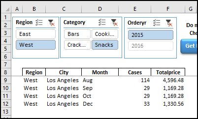
Here’s a screen shot of my original Advanced Filter with Slicers worksheet. Select one criterion from each Slicer, or clear a Slicer, then click a button to run the Advanced Filter. The matching data is shown in the output area.
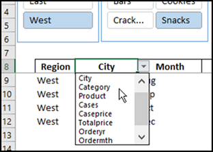
One thing that you might not notice right away — the headings in the output range are drop down lists, so you can choose any fields that you want from the source data.
Advanced Filter Slicers On Demand
In my original file, the Slicers were pretty small, because each field only had 2 or 4 items. In a real-life setting, your data fields probably have many more items than that.
That’s what inspired AlexJ to create a “Slicers on Demand” version for this technique – he needed several Slicers, and each one had many items. There wasn’t room on the worksheet for all of the Slicers, so AlexJ added a bit of code, to make the Slicers appear when needed.
See the Slicers Appear
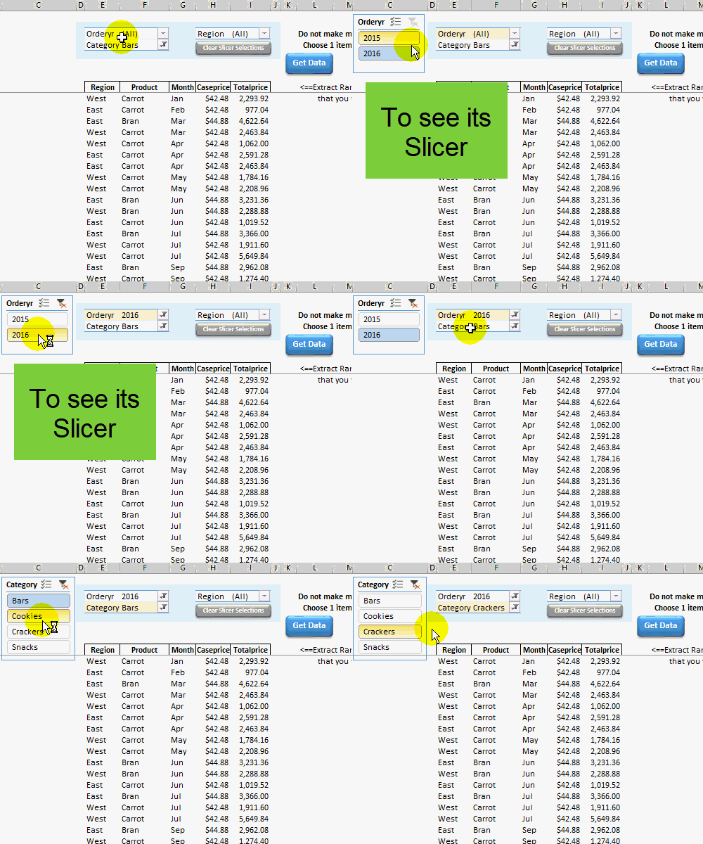
This animated screen shot shows how to make the Slicers appear, by clicking one of the pivot table filter fields. The selected field is highlighted too, to make it stand out on the worksheet. Then, click a different field, to see its Slicer.
How the Slicers Appear
You might have seen AlexJ’s Pop Up Slicers workbook, a couple of weeks ago – it had one Slicer, grouped with macro buttons. This week’s technique is simpler to set up, but has the same result – the Slicers only appear when you need them.
When you click on a pivot table filter field, the Slicer for that field appears.
There is code that runs when you select a cell on the worksheet.
- If the selected cell is in a pivot table (like the pivot table filters here), the code gets the name of the pivot field.
- Then, a macro checks the shapes on the worksheet, to see if any have that pivot field name (all the Slicers are named with a “k_” prefix, and the pivot field name)
- If a matching Slicer is found, it is made visible.
Hidden Admin Section
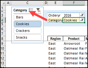
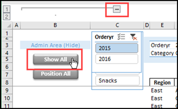
There is a hidden Admin section on the worksheet too. Click the Outline buttons to show that section, if you want to adjust the Slicers.
There are two buttons to help you manage the Slicer setup:
- Click the Show All button, to make all the Slicers visible. In this screen shot, they are stacked up in column C
- Click the Position All button, to align all the Slicers with the top left corner of the active Slicer
Get the Slicers on Demand Workbook
To see how the Slicers work, go to the AlexJ Sample Files page on my Contextures website. In the Filters & Slicers section, look for FL0004 — Advanced Filter with Slicers on Demand, and click the link to download the file.
The zipped file is in xlsm format, and contains macros. There are notes in the workbook, that explain the file setup, and how the code works.
_____________

