Did you win the big prize? Have you ever picked those winning numbers? If you’re keeping track of lottery ticket numbers, use Excel conditional formatting to highlight the winning numbers in a list. Each week, enter the numbers from the latest draw, and Excel will colour all the cells that have matching numbers. You can use a different colour to highlight the latest lottery number matches. The screen shot below shows an example.
Lottery Ticket List
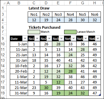
This example will use a named Excel table (tblLottery) to store the lottery ticket purchase history. There is a column for the date, and six columns for the selected numbers. The sheet is named LotteryTable.
In the rows above the table, there are blue cells where the numbers from the latest draw are entered.
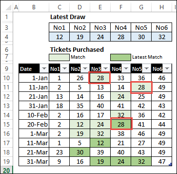
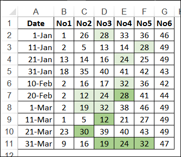
As you can see, all the matching numbers are coloured green, in the Tickets Purchased table. The latest instance of each number is shaded with a darker green.
Conditional Formatting for Matches
The first conditional formatting rule shades all the matching number cells, using light green.
To apply the formatting:
- Select cells C10:H19 – the number cells in the table.
- On the Excel Ribbon, click the Home tab, then click Conditional Formatting
- Click New Rule, to open the New Formatting Rule window
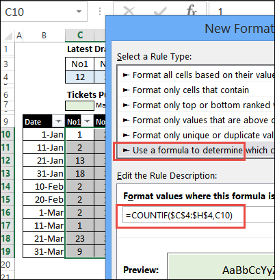
- In the Select a Rule Type list, click Use a formula to determine which cells to format
- Click in the Rule Description box, and type the following formula, to check for matched numbers:
=COUNTIF($C$4:$H$4,C10)
- Click the Format button, and on the Fill tab, click light green
- Click OK, then click OK to close the New Formatting Rule window
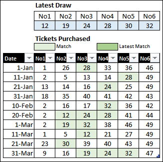
All the cells that match the selected numbers are shaded with light green.
Set Up the Named Ranges
It’s a little more complicated to highlight the latest instance of each number. To make it easier, we’ll create a couple of named ranges.
- Number06 – the table column with the 6th number (No6)
- NumberCheck – all the number cells, starting at the active cell’s row
To create the Number06 named range:
- Select all the numbers in the No6 column in the table
- Click in the Name Box, at the left of the Formula Bar
- Type the name, Number06
- Press Enter, to complete the name
To create the NumberCheck named range:
- Select cell C10, which contains the first number in the table
- On the Excel Ribbon, click the Formula tab, then click Define Name
- Type the name, Number06
- Enter the formula in the Refers To box:
=LotteryTable!$C10:INDEX(Number06,COUNT(Number06),1)
- Click OK to complete the name
Test the NumberCheck Range
The NumberCheck named range was set up with a relative reference for the starting row ($C10). It ends in the last number cell (cell H19), in the No6 column.
To test the range:
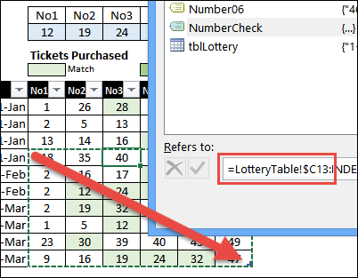
- Select cell E13
- On the Excel Ribbon, click the Formula tab, then click Name Manager
- In the list, click on NumberCheck
- Click anywhere in the Refers To box
- A dashed line will appear around the named range on the worksheet, starting in cell C13, and ending in H19
- The formula has changed, and shows $C13 as the starting cell
- Click Close
Add the Latest Match Conditional Formatting
If a number matches the latest set of numbers drawn, it will be shaded light green, based on our first conditional formatting rule.
COUNTIF($C$4:$H$4,C10)
We’ll add a second rule, that counts how many time the number appears in its NumberCheck range.
COUNTIF(NumberCheck,C10)=1)
If the number only appears once (=1) in the NumberCheck range, then the cell is the latest match. There will never be duplicate numbers in the same row, because you pick 6 unique numbers for your lottery ticket.
To apply the formatting:
- Select cells C10:H19 – the number cells in the table.
- On the Excel Ribbon, click the Home tab, then click Conditional Formatting
- Click New Rule, to open the New Formatting Rule window
- In the Select a Rule Type list, click Use a formula to determine which cells to format
- Click in the Rule Description box, and type the following formula, to check for matched numbers, and instances in the NumberCheck range:
=AND(COUNTIF($C$4:$H$4,C10),COUNTIF(NumberCheck,C10)=1)
- Click the Format button, and on the Fill tab, click medium green
- Click OK, then click OK to close the New Formatting Rule window
Any cell that has the latest match for a selected number is shaded with medium green.
In the screen shot below, the number 28 is found in rows 10, 11 and 15. The first two are light green, and the third instance is medium green.
Download the Sample File
To download the sample file, go to the Conditional Formatting Examples page on my Contextures website. Then, go to the Download section, to get the file.
This example is on the LotteryTable worksheet, and there is a similar example on the LotteryList sheet, for a non-table list.
_______________

I have a formula =COUNTIFS($R3:$AK,B3). It is highlighting the matching lottery numbers in columns B through F but not highlighting the matching numbers and column’s G through K.
Thanks, Toni, and if the winning numbers are listed in cells R3 to AK3, that range should have 4 dollar signs in the conditional formatting formula.
• =COUNTIFS($R$3:$AK$3,B3)
And when you create the conditional formatting rule,
• if your ticket numbers are in cells B3 to K10,
• be sure to select all those cells,
• starting from cell B3, down and across to K10