Change Single Column List to 2 Column Table

Change Single Column List to 2 Column Table

On the weekend, I copied a list of blog names and URLs into Excel. On the website that I copied it from, the list was in 2 columns, but it pasted into a single column in Excel. Having everything mixed together in one column wasn’t going to be very helpful. Here’s what I did to change single column list to 2 column table.

Add Headings and IDs

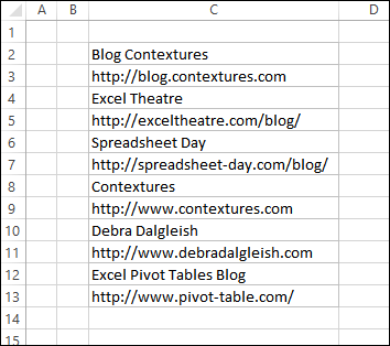
This screen shot shows the list, in a single column.
sortalternaterows09

I wanted the site names in one column, and the URLs in another. If I labeled all the site names as “a”, and the URLs as “b”, I’d be able to sort them into two groups.

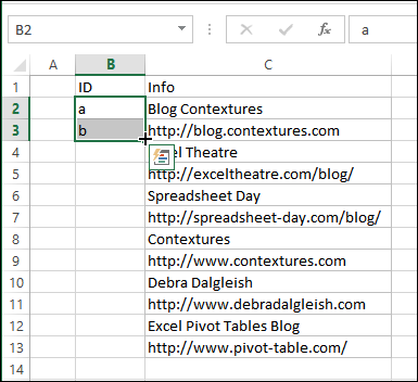
  • First, I put a heading at the top of the list, and an “ID” heading for the column to the left.
  • Then, I typed “a” and “b” as the IDs for the first two rows.

NOTE: if your data is in groups of three or more rows, give a unique letter ID to each item in the first group.
sortalternaterows01

Fill the ID Column

To label the remaining rows, fill the IDs down:

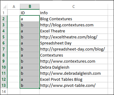
  • Select the first two IDs
  • Point to the Fill Handle – the small black square at the bottom left of the selected range
  • When the pointer changes to a black plus sign, double-click
  • The IDs will fill down, stopping above the first blank row.
sortalternaterows02

Sort by ID

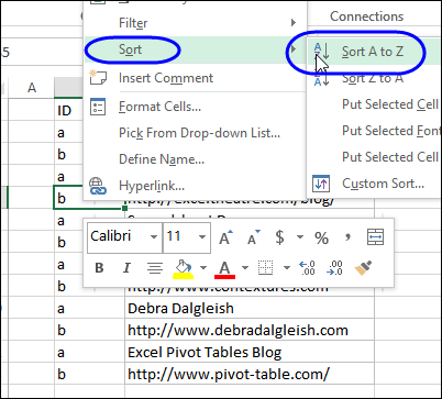
  • Next, right-click a cell in the ID column
  • Click Sort, then Sort A to Z

This will group the data by type – all the site names are listed first, followed by all the URLs.
sortalternaterows03

Move the URLs

To put the data side-by-side:

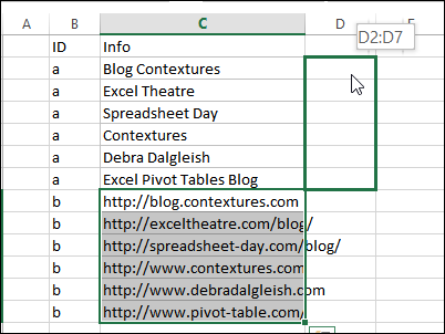
  • Select all the URL cells
  • Drag them up to the column to the right of the site names. Be sure to drop them beside the first row of data.
sortalternaterows04

Create a Formatted Table

Now that all the data is in the correct place, the final steps will change the two column list into a formatted table.

  • Delete the ID column, and add a heading to each column

sortalternaterows05

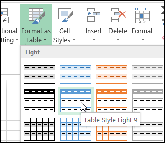
  • Select a cell in the table, and on the Home tab of the Ribbon, click Format as Table.
  • Click on a Table style, to create the table.
sortalternaterows06

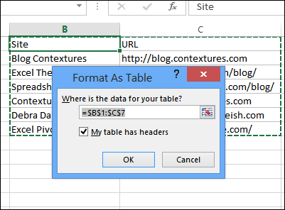
When the Format as Table dialog box appears, check the data range, and correct it, if necessary

Add a check mark to “My table has headers”, and click OK
sortalternaterows07

Now the table is nicely formatted, and you can add new items to the bottom of the list, and the table will expand automatically to include them. You can read more about Excel tables on my website.

sortalternaterows08

Other Ways to Fix the List

If you have a different solution, please let me know in the comments. Maybe there’s an even easier way to do this.
__________________

14 thoughts on “Change Single Column List to 2 Column Table”

  1. Debra, I need to do this often, and use a variation of your a & b sorting trick.
    One additional thing I do is to add a “REC_NUM” column, and insert serial numbers before doing in any such sorting or splitting.
    I prefer to put ‘001 (with single quote prefix) in the first record, and then double-click on the fill handle.
    This helps to easily re-sort the data back to its original form, in case something goes wrong.

      1. You’re welcome Debra 🙂
        In fact, I use this technique in almost any situation where I need to analyze a bunch of records — whether they may need to be sorted or not. It has saved me a lot of time over the years.

  2. Dear Debra,
    You have raised an interesting task and your solution seems to me an optimal one
    However I aimed to find an alternative, non-programmed and non-formula solution (just for sportive interest). It seems that I have succeeded with the following steps:
    1) We select the single column table and turn it to the Table (Insert -> Table -> Create Table -> OK). By default (Excel 2007) the Table is formatted with a style with “Banded Rows” on
    2) We select the Table, copy it, then go to MS Word and make Paste there
    3) Then we select MS Word Table, copy it, then go back to MS Excel and Paste it there
    4) Then we apply an ordinary AutoFilter to the latter table and here we are able to filter by colours (the ones are inherited from banded rows)
    5) Last steps are obvious: to filter every other colour and paste records to another location as column-by-column
    Thus we have turned a single column table into two columns
    I understand that this way is not a perfect; it is more like a kind of a workaround. Anyway we can consider such theoretical non-formula alternative as well…

    1. Ivan, you don’t need to do the copy-paste into Word and back into Excel.
      Once you have converted the data into a Table, just convert it back to a range (Table Tools > Convert to Range > Yes).
      The Table formatting is retained, and you can resume from step 4 in your comment 🙂

  3. Hi Debra
    Nice article.
    Another way to get the data into the two columns would be as follows.
    1. Don,t bother to fill column B with “a”‘s “b”‘s
    2. In D2 enter =INDEX($C$2:$C$13,(ROW()-1)*2-1) and copy down through D3:D7
    3. In E2 enter =INDEX($C$2:$C$13,(ROW()-1)*2) and copy down through E3:E7
    4. Copy D2:E7 and Paste Special > Values to D2
    5. Delete column C and then format as table as per your instructions.

  4. Hi Debra,
    Just amazes me with the kind of content you keep churning out… Thanks,as usual for another great trick.
    I tried Roger’s solution. It works perfectly but for the fact if any rows are entered above this series.
    What is the fix to retain the formulae considering rows are entered above the data set?
    Thanks,
    Adi

  5. The problem that using the function row() brings up is exactly the one that Adi mentions. When i faced this problem, i opted to use a new table with a series of numbers. In the example below, suppose a data table with groups of 2 items per record, but i used it to fix groups of 30 items per record, just changing 2 to 30. Note that $A2 should be an empty cell.
    A B C
    1 2
    Name Id #
    1 =INDEX(Data!$A:$A,B$1+($A2*2),) =INDEX(Data!$A:$A,C$1+($A2*2),)
    2
    3
    4
    5

  6. ASAP Utilities – an Excel add on – allows you to do transpose one column of data into any number of columns with just a couple of mouse clicks.

  7. Here’s another easy cleanup suggestion, from Don Brockett — just copy and paste, then delete the unnecessary rows:
    Copy the mixed data into successive columns, but with each successive column one row higher (or lower) than the predecessor.
    Then it’s simply a matter of deleting the rows that have the junk data.
    The junk rows can be selected in a variety of ways, depending on the content of the data. In your example, all rows in the “C” column that start with “http” would work.

Leave a Reply

Your email address will not be published.

This site uses Akismet to reduce spam. Learn how your comment data is processed.