Happy Halloween! It’s the day for tricks and treats, so here is a useful trick that you can use with your drop down lists.
We’ll block changes in Excel drop down list cells, and that could prevent your worksheet’s data from turning into a nightmare!
Greatest Horror Films List
To show how this trick works, I used the movies from the Horror section in The Guardian’s Greatest Films spreadsheet.
- Fun Fact: I used the same movies a couple of Halloweens ago, to show how Slicers work.
About half of the horror movies were made in the USA, so to keep things simple, I grouped the countries as USA and Other.
And let’s see how many of those horror movie titles I can use in the instructions below! Can you spot them all?
Let the Right One In
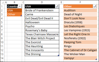
To show how this trick works, I set up list of countries (USA and Other), then a list of the top horror films made in each of those countries.
The Exor-List
The data in each list is named:
- ListCountry
- ListOther
- ListUSA
On the Data Entry sheet, I added a data validation drop down in column B, based on the ListCountry range.
In column C, I created another drop down, and it uses the INDIRECT function to create a range reference:
- =INDIRECT(“List” & B2)
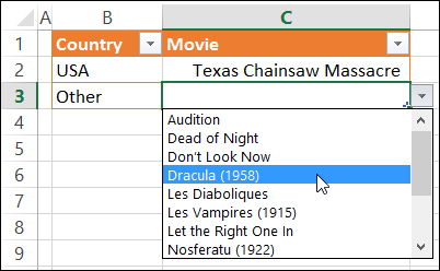
In the screen shot below (or is it a “scream” shot?):
- USA is selected in cell B2, so the drop down in C2 shows the items in the range named ListUSA.
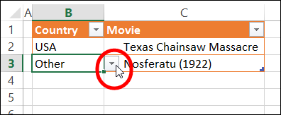
- Other is selected in cell B3, so the drop down in C3 shows the items in the range named ListOther.
Don’t Look Now
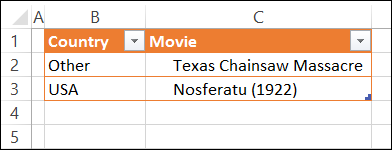
Things can go wrong though, if someone goes back to the Country cell, and changes it. Then, the country and movie selections are mismatched .
For example, Country is changed to Other, and Texas Chainsaw Massacre is selected in the second column. Oh, the horror!
Evil Dead
Fortunately, we can prevent this kind of evil activity, by changing the data validation formula in the Country column.
Currently, the formula just refers to the country list: =ListCountry
I’ll change the formula, so it checks to see if the movie cell is empty.
Let the Right One In
With the revised formula, if the cell is empty, it will show the ListCountry items.
- =IF(C2=””,ListCountry,
If the movie cell is not empty, it will try to show the items in the range named “FakeRange”.
- I can’t use that name on its own in the formula, because Excel will detect that the range doesn’t exist.
- So, I’ll use it with INDIRECT, and Excel will let me enter the formula.
If C2 has an entry, Excel will warn me about the error, but I can click “Yes” in the message, to ignore it.
=IF(C2=””,ListCountry,INDIRECT(“FakeRange”))
Les Diaboliques
Back on the worksheet, I’ll click the drop-down arrow in cell B3 again.
- There isn’t any range named “FakeRange” in this workbook
- So, the formula result is an error, and the drop down list doesn’t work.
- The cell’s drop-down arrow appears, but nothing happens when you click on it.

Ha! We are truly Les Diaboliques!
But don’t worry. We’re doing this to protect The Innocents, who might accidentally mess up our worksheets in the Dead of Night.
Video: Block Changes in Excel Drop Down List
Watch this short video to see how this technique works, and see how to set up the data validation in both columns.
Download the Sample File
To download the sample file, please visit the Advanced Dependent Data Validation page on my Contextures website.
The zipped file is in Excel xlsx format, and there are no macros in the file.
_______________

What a wonderful trick!!
Happy Halloween
Thanks great trick Debra!
Just crazy! I never knew that this could be done.
Thank you!
Your “MAC List” with the apples is funny. LOL
Hi,
I need help at part “Block Changes in Excel Drop Down List”. I did everything as you described, but when I click OK at the end , the Formula error message pops-up. Where did I go wrong?
Thanks in advance