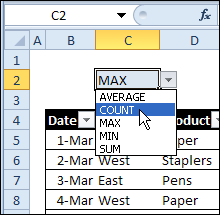
A couple of years ago, we looked at the Excel SUBTOTAL function, and saw how you could allow users to select the function they want. In the example shown below, the total formulas are controlled by the drop down list at the top of the sheet.
Today, we’ll use a similar technique to change functions with AGGREGATE – one of Excel’s newer functions.
Select a Function for SUBTOTAL
This screen shot shows the drop down list of functions that people could choose from, for a SUBTOTAL formula.
The AGGREGATE Function
In Excel 2010 the AGGREGATE function was introduced, and it’s like a supercharged version of SUBTOTAL.
AGGREGATE has a longer list of functions, plus options on what data, if any, to ignore.
-
- For some functions, you can use the Reference form, with these arguments:
- AGGREGATE(function_num, options, ref1, [ref2], …)
- For a few functions, such as LARGE, you can use the Array form, with these arguments:
- AGGREGATE(function_num, options, array, [k])
- For some functions, you can use the Reference form, with these arguments:
Make AGGREGATE Easier
To make AGGREGATE easier to use, I’ve created a sample file that lets you select:
- a function
- an option for what to ignore
- a [k] setting, for the array functions.
Set Up the Data
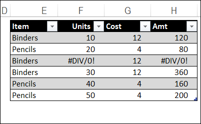
In this example, there are sales orders, in a formatted Excel table named tblSales. There is an error in one of the rows, and you will be able to ignore that, if you choose to.
List the AGGREGATE Functions and Options
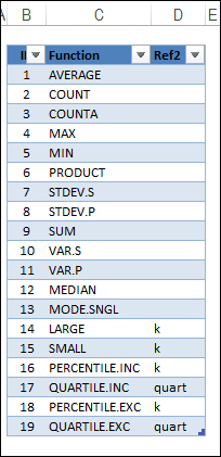
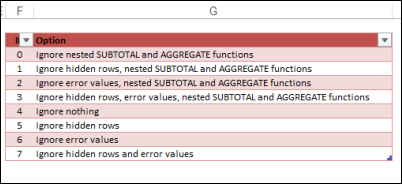
In the Excel Help for AGGREGATE, you’ll find a list of the functions and their numbers. There is also a list of the options for what to ignore.
I’ve put those lists into the sample workbook, as formatted tables. Then, I named the columns in each table, so I could use them in the formulas. For example, the column with function names is FunctionsList.
There are 19 functions, and the third column shows which ones require the [k] argument
There are 8 options for ignoring data.
Create Drop Down Lists
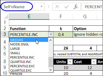
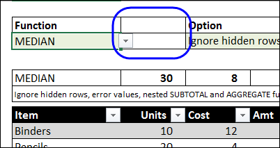
On the sales order sheet, above the Excel table, create drop down lists of functions and options, by using a data validation list. Between them, there is a cell where the k value can be typed, when it is required.
These cells are named – SelFnName, SelRef2, and SelOpt.
Set Default Function and Option Numbers
The AGGREGATE function needs a number, not a function or option name. To find the numbers, you can use the INDEX function with MATCH.
First, I selected default functions and options, just in case the drop down lists are cleared out.
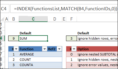
In cell B4 of the lists sheet, I typed a 9, and in cell C4, used INDEX and MATCH to show the function name. There is a similar setup for the Options, in cells F4:G4.
Here is the formula in cell C4:
- =INDEX(FunctionsList,MATCH(B4,FunctionIDs,0))
Cell B4 is named FunctionDefault and F4 is named OptionDefault.
Find the Selected Function and Option Number
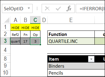
Next, on the orders sheet, use the INDEX function, to find the IDs for function and option, and see if a Ref2 is required. These formulas go into cells A3:C3, and those columns will be hidden.
- In cell A3: =IFERROR(INDEX(FunctionsRef2List, MATCH(SelFnName, FunctionsList,0)),””)
- In cell B3: =IFERROR(INDEX(FunctionIDs, MATCH(SelFnName, FunctionsList,0)), FunctionDefault)
- In cell C3: =IFERROR(INDEX(OptionIDs, MATCH(SelOpt, OptionsList,0)), OptionDefault)
These cells are named as Ref2ID, SelFnID and SelOptID.
Create the Subtotal Formulas
Above the table, we’ll use formulas to calculate the totals for the Units, Cost and Amt columns.
Here is the formula in cell F5, which is copied across to H5:
- =IF(Ref2ID=0, AGGREGATE(SelFnID, SelOptID, tblSales[Units]),
AGGREGATE(SelFnID, SelOptID, tblSales[Units], SelRef2))
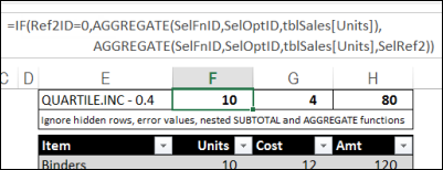
First, the formula checks for a Ref2ID.
- If there isn’t one (=0), the first version of the AGGREGATE formula is used – AGGREGATE(SelFnID,SelOptID,tblSales[Units])
- If there is a RefID, the second version of the formula is used – AGGREGATE(SelFnID,SelOptID,tblSales[Units],SelRef2)
To show what was selected, the formula in cell E5 combines the function name and k value, if any:
=SelFnName & IF(A3=0,””,” – ” & F3)
In cell E6, there is a simple link to the selected option: =SelOpt
Test the Drop Downs
To test the drop downs, filter the Item column in the sal
es table, to hide one of the items. Then, select a function name and option, and enter a k value, if required. There is conditional formatting on the k value cells, so they don’t appear if not required.
The total cells will automatically change, to show the totals for the selected function and option.
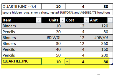
NOTE: In the sample file, the same formulas are in the tables Total row. To see that, select a cell in the table and click the Design tab on the Ribbon. Add a check mark to Total Row. I turned this off in the sample file because the drop down arrows in that row make it very easy to overwrite the formulas.
Download the Sample File
To see the function, and the lists, you can download sample file. On my Contextures website, go to the Sample Files page, and in the Functions section, look for FN0030 – Flexible AGGREGATE Function Selector.
The file is in xlsx format, and is zipped. There are no macros in the workbook.
_________________

Please check the sample file. Some of the names on the Lists sheet point to a file on your harddrive and result in a “missing links” error. Thank you.
@Ute-S, thanks, it’s fixed now.