

Use INDEX and MATCH together, for a powerful lookup formula. It’s similar to a VLOOKUP formula, but more flexible — the item that you’re looking for doesn’t have to be in the first column at the left. Watch the video to see how it works (there are written instructions too), and download the sample workbook to follow along.
Excel Lookup With Two Criteria
Watch this video to see how INDEX and MATCH work together — first with one criterion, and then with multiple criteria. Download the sample workbook to follow along, and the written instructions are below the video.
- 0:00 Introduction
- 0:26 Lookup with One Criterion
- 1:52 Test Each Criterion
- 2:22 Test With a Formula
- 3:26 Multiply the Results
- 4:03 INDEX / MATCH Formula
- 5:20 Check the Formula
- 5:57 Get the Sample File
Get Item Price with INDEX and MATCH
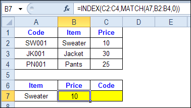
To see how INDEX and MATCH work together, we’ll start with an example that has only 1 criterion. Our price list has item names in column B, and we want to get the matching price from column C.
In the screen shot below, cell A7 has the name of the item that we need a price for – Sweater.
We can enter an INDEX and MATCH formula in cell C7, to get the price for that item:
=INDEX($C$2:$C$4,MATCH(A7,$B$2:$B$4,0))
How the INDEX and MATCH Formula Works
Here’s how the two functions work together:
- MATCH function gets the location of an item in a list
- INDEX function returns a value from a specific location in a list.
So, in our formula:
- the MATCH function looks for “Sweater” in the range B2:B4.
- The result is 1, because “Sweater” is item number 1, in that range of cells.
- the INDEX function looks in the range C2:C4
- The result is 10, from row 1 in that range
So, by combining INDEX and MATCH, you can find the row with “Sweater” and return the price from that row.
Find a Match for Multiple Criteria
In the first example, there was only one criterion, and the match was based on the Item name – Sweater. However, sometimes life, and Excel workbooks, are more complicated.
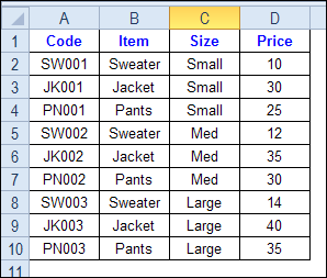
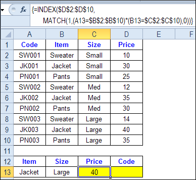
In the screen shot below, each item is listed 3 times in the pricing lookup table. We want to find the price for a large jacket.
To get the right price, you’ll need to use 2 criteria:
- the item name
- the size
Does it MATCH? True or False
Instead of a simple MATCH formula, we’ll use one that checks both the Item and Size columns.
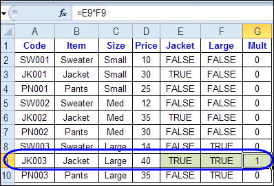
To see how this formula will work, I’ll temporarily add columns to check the item and Size of each item — is the item a Jacket, and is the Size a Large?
Enter this formula in E2, and copy down to E10: =C2=$C$13
Enter this formula in F2, and copy down to F10: =D2=$D$13
- If the Item in column B is a Jacket, the result in column E is TRUE. If not, the result is FALSE
- If the Size in column C is Large, the result in column F is TRUE. If not, the result is FALSE
To see if both results are TRUE in each row, enter this formula in G2, and copy down to G10: =F2*G2
When you multiply the TRUE/FALSE values,
- If either value is FALSE (0), the result is zero
- If both values are TRUE, the result is 1
Only the 8th row in our list of items has a 1, because both values are TRUE in that row.
We can tell the MATCH function to look for a 1, and that will return the information that we need.
Use MATCH With Multiple Criteria
Instead of adding extra columns to the worksheet, we can use an array-entered INDEX and MATCH formula to do all the work.
Here is the formula that we’ll use to get the correct price, and the explanation is below:
=INDEX($D$2:$D$10,
MATCH(1,(A13=$B$2:$B$10) * (B13=$C$2:$C$10),0))
NOTE: This is an array-entered formula, so press Ctrl + Shift + Enter, instead of just pressing the Enter key.
How the Formula Works
In this INDEX and MATCH example,
- prices are in cells D2:D10, so that is the range that the INDEX function will use
- the item name is in cell A13
- the size is in cell B13.
The formula checks for the selected items in $B$2:$B$10, and sizes in $C$2:$C$10. The results are multiplied.
- (A13=$B$2:$B$10)*(B13=$C$2:$C$10)
The MATCH function looks for the 1 in the array of results.
- MATCH(1,(A13=$B$2:$B$10)*(B13=$C$2:$C$10),0)
If you select that part of the formula and press the F9 key, you can see the calculated results. In the screen shot below there are 9 results, and all are zero, except the 8th result, which is 1.
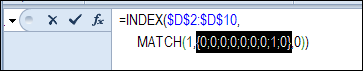
So, the INDEX function returns the price – 40 – from the 8th data row in column D (cell D9).
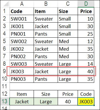
Get the Product Code
To find the product code for the selected item and size, you would change the formula to look in cells A2:A10, instead of the price column.
Put this formula in cell D13, and remember, this is an array-entered formula, so press Ctrl + Shift + Enter.
=INDEX($A$2:$A$10,
MATCH(1,(A13=$B$2:$B$10) * (B13=$C$2:$C$10),0))
In this example, the product code would be JK003, from cell A9.
Get the Workbook
To get the sample file with the Lookup Multiple Criteria examples, go to the Excel Lookup Multiple Criteria page on my Contextures site.
For more INDEX and MATCH tips and examples, visit the INDEX function and MATCH function page on the Contextures website. This is Example 4 in the sample file section of that page.
_____________
It is helpful.
but You are returning a value based on and conditions.
but how to return a value based on OR condition .
DB:
Sankar Y
Senthil Y
Sankar Y
Vinod N
Gokul Y
Senthil N
Should return a Values which name is either (Senthil and Y)–If anyone Condition Satisfies means it has to return
Hello,
I have trouble using the INDEX & MATCH with multiple criteria.
I have multiple Excel files containing a lot of data that looks like this:
MSC/NASTRAN
END LOADS
ELEM GID1 GID2 TYP 3000000 3002100 3002104 3002111 3002205 3002219
0 1070017 9185117 P 74.1 2.2 82.8 74.2 21.3 57.8
0 1070017 9185118 P 98.4 82.4 10.8 0.3 21.4 72.5
0 1070018 9185114 P 74.6 43.1 18 86.4 19 32.2
0 1070018 9185115 P 22.5 41.6 74 98.1 58.9 28.9
0 1070019 9185113 P 87.5 14.9 63.6 92.7 26.2 37.9
0 1070020 9185112 P 34 11.1 83 51.6 66.5 59.1
0 1070067 9185116 P 99.9 76 61.1 23.5 2.8 79.7
0 1070517 9185617 P 35.3 82.4 63.4 7.5 36.8 55.5
0 1070517 9185618 P 11.6 70.7 89.7 17.3 95.4 29.5
0 1070518 9185614 P 16.7 66 87.1 31.4 10 48.5
0 1070518 9185615 P 49.5 72.9 62.5 68.3 93.6 51
0 1070519 9185613 P 18.4 0.9 51.6 20.3 72.2 6.5
Please note that this file contains thousands of rows and hundreds of columns…
In a separate file that I call EXTRACTOR, I want to extract data from the previous file.
There are 4 criteria that I want to check: ELEM, GID1, GID2 AND TYP
In the EXTRACTOR, the user has to specify the name of the file from where he wants to extract data. He is also asked to give then name of the sheet (please note that the file containing the data has to be open)
Name of file containing all loads (with correct extension): loads.xlsx
Name of sheet containing all loads: sheet1
Then I do a CONCATENATE of these 2 entries in cell N6 (in EXTRACTOR) in order to have: [loads.xlsx]sheet1!
This will be used further in cell E12 formula…
Now, in EXTRACTOR, I type (starting at cell A11):
ELEM GID1 GID2 TYP 3000000 3002100 3002104 3002111 3002205 3002219
0 1070017 9185117 P #N/A
Cell E12 displays “#N/A” and contains the following big formula:
= INDEX(
CONCATENATE($N$6, ADDRESS(6, COLUMN(E10),2),”:”, ADDRESS(15000, COLUMN(E10),2) ),
MATCH(1,
($A12= CONCATENATE($N$6,”$A$6:$A$15000″) )
*
($B12= CONCATENATE($N$6,”$B$6:$B$15000″) )
*
($C12= CONCATENATE($N$6,”$C$6:$C$15000″) )
*
($D12= CONCATENATE($N$6,”$D$6:$D$15000″) ),0),1
)
This formula doesn’t seem to work properly…
When I do EVALUATE FORMULA, I get FALSE in every MATCH criteria check, which in the end gives me #N/A within the MATCH, and also #N/A for the global formula
I hope my description of the problem is clear enough.
If somebody can help, it would be very very appreciated!
By the way, using MS Excel 2010 on XP 64 bits
Thank you!
J.
Hi, This is a very helpful tutorial. I was wondering that, how I can use Match function to find a value in a range of cells between certain values such as,
=INDEX($A$4:$A$12,MATCH(1,(G13>=$E$4:$E$12)*(G13<=$F$4:$F$12),0)). Thanks in advance
I’ve used the index/match array version to lookup multi-critreria data and it works great! However, I’m experiencing a problem when sorting on columns outside the column that contains the array formula. It seems as if the relative cell references do not follow the sort. Can anyone help or explain why this may happen?
Thanks!
@Josh: Can you post a sample workbook somewhere, or explain a little bit more fully what your data looks like and what you are trying to do?
@Joaquim: This is a little hard to conceptualize. Can you post a sample workbook somewhere and post the link here?
@Jeff: Thank you for your reply! I will provide such a sample at the beginning of next week. Thanks again 🙂
P.S.: Any suggestion where to put the sample?