

Use INDEX and MATCH together, for a powerful lookup formula. It’s similar to a VLOOKUP formula, but more flexible — the item that you’re looking for doesn’t have to be in the first column at the left. Watch the video to see how it works (there are written instructions too), and download the sample workbook to follow along.
Excel Lookup With Two Criteria
Watch this video to see how INDEX and MATCH work together — first with one criterion, and then with multiple criteria. Download the sample workbook to follow along, and the written instructions are below the video.
- 0:00 Introduction
- 0:26 Lookup with One Criterion
- 1:52 Test Each Criterion
- 2:22 Test With a Formula
- 3:26 Multiply the Results
- 4:03 INDEX / MATCH Formula
- 5:20 Check the Formula
- 5:57 Get the Sample File
Get Item Price with INDEX and MATCH
To see how INDEX and MATCH work together, we’ll start with an example that has only 1 criterion. Our price list has item names in column B, and we want to get the matching price from column C.
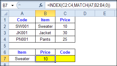
In the screen shot below, cell A7 has the name of the item that we need a price for – Sweater.
We can enter an INDEX and MATCH formula in cell C7, to get the price for that item:
=INDEX($C$2:$C$4,MATCH(A7,$B$2:$B$4,0))
How the INDEX and MATCH Formula Works
Here’s how the two functions work together:
- MATCH function gets the location of an item in a list
- INDEX function returns a value from a specific location in a list.
So, in our formula:
- the MATCH function looks for “Sweater” in the range B2:B4.
- The result is 1, because “Sweater” is item number 1, in that range of cells.
- the INDEX function looks in the range C2:C4
- The result is 10, from row 1 in that range
So, by combining INDEX and MATCH, you can find the row with “Sweater” and return the price from that row.
Find a Match for Multiple Criteria
In the first example, there was only one criterion, and the match was based on the Item name – Sweater. However, sometimes life, and Excel workbooks, are more complicated.
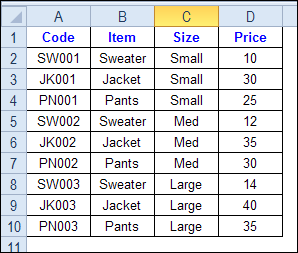
In the screen shot below, each item is listed 3 times in the pricing lookup table. We want to find the price for a large jacket.
To get the right price, you’ll need to use 2 criteria:
- the item name
- the size
Does it MATCH? True or False
Instead of a simple MATCH formula, we’ll use one that checks both the Item and Size columns.
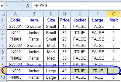
To see how this formula will work, I’ll temporarily add columns to check the item and Size of each item — is the item a Jacket, and is the Size a Large?
Enter this formula in E2, and copy down to E10: =C2=$C$13
Enter this formula in F2, and copy down to F10: =D2=$D$13
- If the Item in column B is a Jacket, the result in column E is TRUE. If not, the result is FALSE
- If the Size in column C is Large, the result in column F is TRUE. If not, the result is FALSE
To see if both results are TRUE in each row, enter this formula in G2, and copy down to G10: =F2*G2
When you multiply the TRUE/FALSE values,
- If either value is FALSE (0), the result is zero
- If both values are TRUE, the result is 1
Only the 8th row in our list of items has a 1, because both values are TRUE in that row.
We can tell the MATCH function to look for a 1, and that will return the information that we need.
Use MATCH With Multiple Criteria
Instead of adding extra columns to the worksheet, we can use an array-entered INDEX and MATCH formula to do all the work.
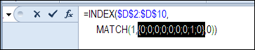
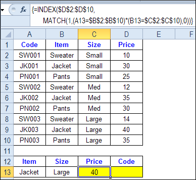
Here is the formula that we’ll use to get the correct price, and the explanation is below:
=INDEX($D$2:$D$10,
MATCH(1,(A13=$B$2:$B$10) * (B13=$C$2:$C$10),0))
NOTE: This is an array-entered formula, so press Ctrl + Shift + Enter, instead of just pressing the Enter key.
How the Formula Works
In this INDEX and MATCH example,
- prices are in cells D2:D10, so that is the range that the INDEX function will use
- the item name is in cell A13
- the size is in cell B13.
The formula checks for the selected items in $B$2:$B$10, and sizes in $C$2:$C$10. The results are multiplied.
- (A13=$B$2:$B$10)*(B13=$C$2:$C$10)
The MATCH function looks for the 1 in the array of results.
- MATCH(1,(A13=$B$2:$B$10)*(B13=$C$2:$C$10),0)
If you select that part of the formula and press the F9 key, you can see the calculated results. In the screen shot below there are 9 results, and all are zero, except the 8th result, which is 1.
So, the INDEX function returns the price – 40 – from the 8th data row in column D (cell D9).
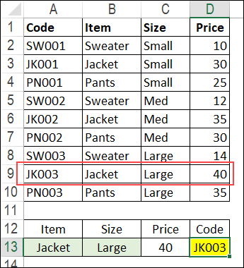
Get the Product Code
To find the product code for the selected item and size, you would change the formula to look in cells A2:A10, instead of the price column.
Put this formula in cell D13, and remember, this is an array-entered formula, so press Ctrl + Shift + Enter.
=INDEX($A$2:$A$10,
MATCH(1,(A13=$B$2:$B$10) * (B13=$C$2:$C$10),0))
In this example, the product code would be JK003, from cell A9.
Get the Workbook
To get the sample file with the Lookup Multiple Criteria examples, go to the Excel Lookup Multiple Criteria page on my Contextures site.
For more INDEX and MATCH tips and examples, visit the INDEX function and MATCH function page on the Contextures website. This is Example 4 in the sample file section of that page.
_____________
I’m running into an issue with this function whereby I have 2 drop down lists of variables to match; one list contains 3 items, the other 2. The function works great for 2 of the list of 3 and 1 of the list of 2. I’ve gone through the formulas 3 times, I’ve checked for spelling errors. I don’t get an #N/A error, no #VALUE error, just nothing comes through when I select one of the variables. When I highlight the formula as described above and look for the 0,0,0,1,0,0…there is no “1” for the list item that is not working. What could possibly be the problem?
The array formula only works where more than one row exists in a table. I’m using a dynamic table where the rows are populated using a query on our SQL Server. The array formula does not work if the result set from the query only returns a single row to the table.
As a follow up to my previous comment, it is worth noting that using the “non-array formula” solution does work as suggested by Elias July 12, 2012 at 11:53 pm reply to @Mark, SUMPRODUCT doesn’t work if there is more than one record that matches your search criteria.
As a regular formula, this worked:
=IFERROR(INDEX(Table_SQL,MATCH(1,INDEX(($A5=Table_SQL[PartNo])*(AK$4=Table_SQL[SerialIndex]),0)),5),””)
The array formula (ctrl-shift-enter) did NOT work when Table_SQL contains 1 result set only (works OK where multiple rows exist):
=IFERROR(INDEX(Table_SQL,MATCH(1,($A5=Table_SQL[PartNo])*(AK$4=Table_SQL[SerialIndex]),0),5),””)
This might be the best excel tip ever. Thanks
Very Helpful! Thanks for sharing!
i want to take average of 3 data sets and consolidate in to 1. for example column a has product list for month of may , column b has the number of tests run, column c has product for month of june, column d has corresponding data: now take an average of two months data ,in this case the products list in a and c column may not be same
Hi, i am looking up an external Table in another spreadsheet. My “Index match” formula only brings back the results when I open the external spreadsheet. Yet an “if” formula for the external spreadsheet always works.
One thing I do notice is that , when i refresh the external link, my index match formula below is not capturing the worksheet name “Cumu” in the file called SWP. I thought the table name got around the need for the worksheet name?
Any ideas why I have to open the external sheet every time and how to capture the Woksheet name please ?
Index Match formula:
=IFERROR(INDEX(‘I:\Pricing\SWP\swp.xlsx’!prices[#All],MATCH([@date],’I:\Pricing\SWP\swp.xlsx’!prices[[#All],[date]],0),MATCH(M$2,’I:\Pricing\SWP\swp.xlsx’!prices[#Headers],0)),””)
“If” formula that always works, and I dont have to open up the SWP spreadsheet.
=IF(‘I:\Pricing\SWP\[swp.xlsx]cumu’!P2048>0,’I:\Pricing\SWP\[swp.xlsx]cumu’!P2048,””)
Thanks for any assistance you can give !!