In an Excel file, you might need to change the layout, before you print a report. For example,
- in a customer report, the pricing columns are hidden.
- for a supplier report, you filter for a specific product, and hide some columns.
- for your internal reports, all the columns and rows are visible.
Create Custom Views
To quickly show the different layouts, without any programming, you can create Custom Views, and select one from a drop down list.
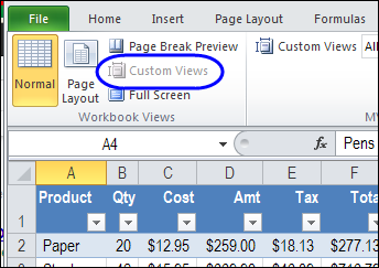
NOTE: In Excel 2007 and Excel 2010, the Custom View options are not available, if there is a named Excel Table, anywhere in the workbook.
Set Up a Default Custom View
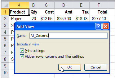
If you’re creating Custom Views, you should create a default Custom View first, with the layout that you use most often. In this example, the default worksheet layout has all the columns and rows visible.
To create a Custom View
- On the Excel Ribbon, click the View tab
- Click Custom Views

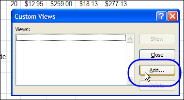
- In the Custom Views dialog box click Add
- Type a name for the Custom View, then click OK
Set Up the Alternate Custom Views
After you set up the default worksheet Custom View, change the layout for the next Custom View. In this example columns C:E are hidden.
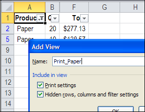
- Click the Custom Views command again, and add a Custom View for this layout – Print_Hidden.
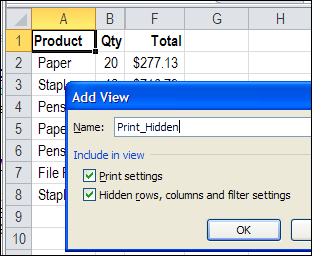
Create as many custom views as you need. This example has a filter applied for paper products, and the Custom View will include those filter settings.
Add a Custom Views List to the Ribbon
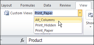
To make it easy to switch between Custom Views, you can add a drop-down list of Custom Views to the Excel Ribbon. (If you’re using Excel 2007, you can add this drop-down list to the Quick Access Toolbar, instead of the Ribbon.)
- In Excel 2010, right-click the Ribbon, and click Customize the Ribbon
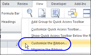
- In the Excel Options window, at the right, click the + to the left of the View tab.
- Click Workbook Views, to select that Group, and click the New Group button. That will add a new Group below Workbook Views.
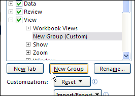
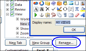
- With the new Group selected, click Rename
- Type a name For the new group, and click OK – in this example the new group is called MY VIEWS
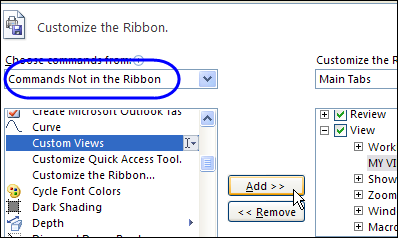
- With the MY VIEWS group selected, click the drop down arrow for Choose Commands From
- Click on Commands Not in the Ribbon
- Scroll down and click on Custom Views, then click Add, to move that command to the MY VIEWS group.
- Click OK, to close the Excel Options window.
Test the Custom Views
On the Excel Ribbon’s View tab, you’ll see the Custom Views drop down list. Select one of the Custom Views to see that layout.

No Excel Tables With Custom Views
Remember though – if you have a named Excel table in your workbook – on any sheet – the Custom Views options will not be available. Strange, but true.
____________

I’ve also noticed that Custom Views do not capture/restore Slicer settings. At least not for powerPivot slicers. You know any way around this limitation? I’ve got VBA code that can save slicer settings and re-apply them, but I was hoping to use custom views to capture and save slicer settings across many slicers… to create custome views of powerPivot reports. (Something similar can be done from sharePoint published powerPivots…)
Thanks for the simple tip. Very well explained as usual.
I saw this thread in yesterday’s email newsletter from Debra, and thought I would share my 2-bits about how I show/hide columns easily.
I use a 1-line VBA macro which toggles the display and hide attributes of columns that I wish to see (or hide).
1. First I setup a range name (say, rShowHideCols) in a row at or near the top of the sheet.
(Make sure it is not part of your data range.)
2. Then I put ‘x’ in all the cells of the range, to indicate columns that I want to keep visible at all times.
The remaining (blank) cells will be used to show/hide their respective columns.
3. AFter that, I insert this bit of code in a module of the workbook:
This code simply toggles the .Hidden property of the columns which have blank cells in the rShowHideCols range.
Sub DoShowHideCols()
ActiveSheet.Range(“rShowHideCols”).SpecialCells(xlCellTypeBlanks).EntireColumn.Hidden = _
Not ActiveSheet.Range(“rShowHideCols”).SpecialCells(xlCellTypeBlanks).EntireColumn.Hidden
End Sub
4. Finally, I assign this macro to a button near the top-left corner of the sheet.
Now whenever I need to see only the relevant (fewer) columns, I click on the button once.
And when I want to see all the columns, I click on the button again.
The advantage of this approach is that I can easily change the columns which I wish to show or hide at any time.
Forgot to mention in my above comment that I use this approach because, for me, the benefits of using Excel tables far outweigh the benefits of using Custom Views. 🙂
I added Custom Views and Custom Views… to the quick access toolbar, then I do not need a My Views group on the View tab of the ribbon. I agree with adding the group if the QAT is getting too crowded however, which is often the case for some.
Thanks Bill!