
Yesterday, in the 30XL30D challenge, we found text strings with the FIND function, and learned that it is case sensitive, unlike the SEARCH function.
INDEX Function
For day 24 in the challenge, we’ll examine the INDEX function. Based on a row and column number, it can return a value or reference to a value. We’ve already used INDEX several times, with other functions in the challenge:
- with EXACT to find name for the password with exact match
- with AREAS to find the last area in a named range
- with COLUMNS to calculate sum of last column in range
- with MATCH to find the name for closest guess in a contest
So, let’s take a look at the INDEX information and examples, and if you have other tips or examples, please share them in the comments.
Function 24: INDEX
The INDEX function returns a value or reference to a value. Combine it with other functions, like MATCH, for powerful formulas.

How Could You Use INDEX?
The INDEX function can return a value or reference to a value, so you can use it to:
- Find sales amount for selected month
- Get reference to specified row, column, area
- Create a dynamic range based on count
- Sort column of text in alphabetical order
INDEX Syntax
The INDEX function has two syntax forms — Array and Reference. With Array form, a value is returned, and with Reference form, a reference is returned.
The Array form has the following syntax:
- INDEX(array,row_num,column_num)
- array is an array constant or range of cells
- if array has only 1 row or column, corresponding row/column number argument is optional
- if array has >1 row or column, and only row_num or column_num is used, array of entire row or column is returned
- row_num – if omitted, column_num is required
- column_num – if omitted, row_num is required
- if both the row_num and column_num arguments are used, returns value in cell at intersection of row_num and column_num
- if row_num or column_num are zero, returns array of values for entire column or row
The Reference form has the following syntax:
- INDEX(reference,row_num,column_num,area_num)
- reference can refer to one or more cell ranges – enclose nonadjacent ranges in parantheses
- if each area in reference has only 1 row or column, corresponding row/column number argument is optional
- area_num selects range in reference from which to return row and column intersection
- area_num – if omitted, area 1 is used
- if row_num or column_num are zero, returns reference for entire column or row
- result is a reference, and can be used by other functions
INDEX Traps
If the row_num and column_num don’t point to a cell within the array or reference, the INDEX function returns a #REF! error.
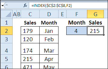
Example 1: Find sales amount for selected month
Enter a row number, and the INDEX function returns the sales amount from that row in the reference. Here the month number is 4, so the April sales amount is returned.
=INDEX($C$2:$C$8,F2)
Find sales amount for selected month
To make the formula more flexible, you could use MATCH to return the row number, based on the month that was selected from a drop down list.
=INDEX($C$2:$C$8,MATCH($F$2,$D$2:$D$8,0))

Example 2: Get reference to specified row, column, area
In this example, there is a named range, MonthAmts, which consists of 3 non-contiguous ranges. The MonthAmts range has 3 areas — one for each month — and there are 4 rows and 2 columns in each area. Here is the formula for the MonthAmts name:
=’Ex02′!$B$3:$C$6,’Ex02′!$E$3:$F$6,’Ex02′!$H$3:$I$6
With the INDEX function, you can return the cost or revenue amount for a specific region and month.
=INDEX(MonthAmts,B10,C10,D10)

The INDEX function result can be multiplied, as in the Tax calculation in cell F10:
=0.05*INDEX(MonthAmts,B10,C10,D10)
or, it can return a reference for the CELL function, to show the address of the result, in cell G10.
=CELL(“address”,INDEX(MonthAmts,B10,C10,D10))

Example 3: Create a dynamic range based on count
You can also use the INDEX function to create a dynamic range. In this example, I’ve created a name, MonthList, with this formula:
=’Ex03′!$C$1:INDEX(‘Ex03’!$C:$C,COUNTA(‘Ex03’!$C:$C))

If another month is added to the list in column C, it will automatically appear in the data validation drop down list in cell F2, which uses MonthList as its source.

Example 4: Sort column of text in alphabetical order
In the final example, the INDEX function is combined with several other functions, to return a list of months, sorted in alphabetical order. The COUNTIF function shows how many month names come before a specific month name. SMALL returns the nth smallest item in the list, and MATCH returns the row number for that month.
In the video, you can see the formula broken down into steps.
This formula is array-entered, by pressing Ctrl + Shift + Enter.
=INDEX($C$4:$C$9,MATCH(SMALL(
COUNTIF($C$4:$C$9,”<“&$C$4:$C$9),ROW(E4)-ROW(E$3)),
COUNTIF($C$4:$C$9,”<“&$C$4:$C$9),0))

Download the INDEX Function File
To see the formulas used in today’s examples, you can download the INDEX function sample workbook. The file is zipped, and is in Excel 2007 file format.
Watch the INDEX Video
To see a demonstration of the examples in the INDEX function sample workbook, watch this short Excel video tutorial.
_____________
Hi Debra,
thanks for your hints.
Two questions linked to the named dynamic range.
1. absolute vs. relative addressing
=$C$1:INDEX(C:C,COUNTA($C:$C)))
there’s a mix of absolute and relative addressing (see the $ signs).
Is this intentionally and necessary?
2. increase the range horizontally
Is it possible to have a named range that spans all the columns of a table?
E.g. to have a dynamic range C4:F9, where the heading might be in C3:F3.
Any solutions?
Hugo, thanks for pointing out the mixed references — that was an error, and it’s fixed now.
Not sure exactly what you want for the table range, but perhaps something like this:
=Sheet1!$C$4:INDEX(Sheet1!$F:$F,COUNTA(Sheet1!$F:$F)+ROW(Sheet1!$F$3)-1)
Hi Debra,
It looks like there is a typo in an “In INDEX Syntax” section.
Instead of “The LOOKUP function has” should be “The INDEX function has”.
It would be easier to follow the article if you show a full definition of MonthAmts named range(screenshot or just a text)
Thank you,
Leonid
Thanks Leonid, I’ve fixed the typo, and added the formula for the MonthAmts named range.
Hi Debra
I mean a kind of this I use very often:
=OFFSET($A$1,,,COUNTA($A:$A),COUNTA($1:$1))assuming, that there’s a table beginning in the upper left corner of the sheet.
Because OFFSET is volotile I would like to substitute this with an INDEX combination.
Can we adapt this to INDEX?
One way, using 30000 as an arbitrary number of rows:
=Sheet1!$A$1:INDEX(Sheet1!$1:$30000,COUNTA(Sheet1!$A:$A),COUNTA(Sheet1!$1:$1))
Hi Debra!
I have learned a lot from this post!
Formula in example 3 also works in a cell, I thought you had to use indirect() or offset() function to return a cell range reference.
=’Ex03′!$C$1:INDEX(‘Ex03’!$C:$C,COUNTA(‘Ex03’!$C:$C))
There is no need anymore for volatile functions like indirect or offset when creating a dynamic array.
Thanks for posting!
Hi Oscar
You’re welcome! Creating a dynamic range with the INDEX function takes a bit of practice, if you’re used to OFFSET, but it’s worth the effort.
[…] bingo workbook, that you could use to create a set of three cards with random numbers. It uses the INDEX and MATCH functions to pull the numbers from another […]
[…] so we’ll create a dynamic range named RateTable, using the technique from Example 3 in the 30XL30D INDEX function […]
[…] we’ll take a closer look at that dynamic range, and see how the INDEX function is used to set the last cell in the […]
Hi Debra!
First of all I want to thank you for all your postings. You’re site has really helped me a lot. I just have a question on hlookup, but I’m afraid to post it here. Can I email you instead? Please give me your email add.
thanks,
@Amee, my email address is on the About page:
ddalgleish AT contextures.com
Hi Debra,
How to calculate composite index?
Hi Debra,
Great Blog!! In Example 03 how were you able to highlight the value in yellow for the returned value??