In Day 4 of the 30XL30D challenge, we got details about the operating environment, with the INFO function — things like the Excel version and recalculation mode.
CELL Function
For day 11 in the challenge, we’ll examine the CELL function, which gives you information about cell formatting, contents and location. CELL is similar to the INFO function, with a list of types that you can enter, but has 2 arguments, instead of only one.
So, let’s take a look at the CELL information and examples, and if you have other tips or examples, please share them in the comments.
Function 11: CELL
The CELL function shows information about formatting, contents and location of the referenced cell.
How Could You Use CELL?
The CELL function can show information about a cell, such as:
- Cell’s number format
- Worksheet name
- Cell alignment or column width
CELL Syntax
The CELL function has the following syntax:
- CELL(info_type,reference)
- info_type is one of the following values
- address…Reference of first cell in reference, as text.
- col…Column # of cell in reference.
- color…1 = color for negative values; otherwise 0 (zero).
- contents…Value of upper-left cell in reference
- coord…Absolute reference of first cell in reference
- filename…Filename and full path
- format…Cell number format
- parentheses…1 = parentheses for positive or all values; otherwise 0.
- prefix …”label prefix” of cell (alignment)
- protect…0 = not locked, 1 = locked.
- row…Row # of cell
- type…type of data in cell (empty, text, other)
- width…Column width of cell
- info_type is one of the following values
CELL Traps
There are a few things to watch for when using the CELL function:
- The CELL function’s reference argument is optional, but if it is omitted, the result is returned for the last cell that was changed. To ensure that the result is what you expect, it’s best to include a reference — you can refer to the cell that contains the CELL formula.
- When using the CELL function, you may need to recalculate the worksheet to update the CELL formula result, if the cell is changed.
- For the “filename” info_type, an empty string is returned if the workbook has not yet been saved.
Example 1: Cell’s Number Format
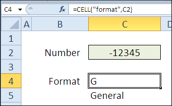
With the “format” value, you can use the CELL function to show the number format of a cell. For example, if cell B7 has General format, the result of this formula is “G”, for General:
=CELL(“format”,C2)
Example 2: Get Worksheet Name
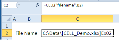
With the “filename” value, the CELL function shows the file path, file name, and worksheet name.
=CELL(“filename”,B2)
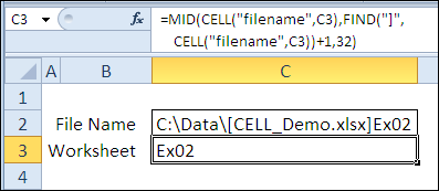
From that result, you can use other functions to extract the worksheet name. In the formula below, the MID and FIND functions are used to find closing square bracket, then return the 32 characters that follow it. (A worksheet name is limited to 31 characters)
=MID(CELL(“filename”,C3),FIND(“]”,CELL(“filename”,C3))+1,32)
Example 3: Get Info_Type From Drop Down
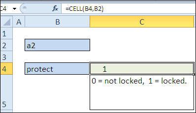
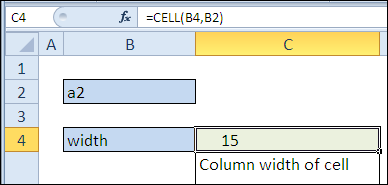
Instead of typing the info_type value as a string in the CELL function, you can refer to a cell that contains one of the valid values. In this example, there is a data validation drop down list in cell B4, and the CELL function refers to it for the info_type value. The cell reference is to B2.
When “protect” is selected, the result is 1 if the cell is locked, and 0 if it’s not locked.
=CELL(B4,B2)
When “width” is selected, the result shows the column width, as an integer. The measurement unit represents the width of one character in the default font size.
Download the CELL Function File
To see the formulas used in today’s examples, you can download the CELL function sample workbook. The file is zipped, and is in Excel 2007 file format.
Watch the CELL Video
To see a demonstration of the examples in the CELL function sample workbook, you can watch this short Excel video tutorial.
YouTube link: Get Excel Worksheet Name With CELL Function
_____________

The =CELL(“filename”) function returns the full file-name along with the sheet name of the active workbook.
This is sometimes not-so-useful to get a ‘clean’ file-name or folder-name
(without the ‘[‘ or ‘]’ or ‘/’ characters).
I use (slightly long) workaround formulas to get the following information:
FILE-NAME of active workbook
=MID((CELL(“filename”)),(SEARCH(“[“,(CELL(“filename”)))+1),(SEARCH(“]”,(CELL(“filename”)))+1)-(SEARCH(“[“,(CELL(“filename”)))+2))
FOLDER / DIRECTORY in which the active workbook is saved
=LEFT((CELL(“filename”)),(SEARCH(“[“,(CELL(“filename”)))-1))
FULL FILE-NAME (with folder name) of the active workbook
=LEFT((CELL(“filename”)),SEARCH(“[“,(CELL(“filename”)))-1)&MID((CELL(“filename”)),(SEARCH(“[“,(CELL(“filename”)))+1),(SEARCH(“]”,(CELL(“filename”))))-(SEARCH(“[“,(CELL(“filename”)))+1))
If there are more efficient formulas, I’d love to hear about them ! 🙂
Khushnood
“When using the CELL function, you may need to recalculate the worksheet to update the CELL formula result, if the cell is changed.”
I think the above is of crucial importance here and it should be noted that this holds true irrespective of Calculation Mode and despite the Functions inherent Volatility.
CELL is one of the “odd ones out” as far as I am concerned.
It is strange that MS offer us a function flawed by it’s specific relationships with non-volatile actions (adjusting number formatting & column widths for ex.).
To the above I would further add that relying on CELL for format related information is also risky if you intend to run a model across multiple locales.
Useful but use at your own risk 😉
[…] CELL […]
I used the Cell() function with a circular reference.
In the blank cell A11, the formula is [=IF(CELL(“type”,A11)=”v”,A10,A11)]
I have to use this formula to copy the content of the upper cell to the current cell.
I enabled Recursive calculation in Options, and expected that the cell will automatically calculate the values – which it did the very first time I entered this in about 2000 cells.
Since that time, I am having to hit F2+Enter for all the remaining cells for the cell to recalculate its value.
I am not able to figure out why does it not autocalculate the formulae the moment I paste it in all empty cells.
Any help appreciated.