A pivot table can sum and count and average, and do several other functions. However, a normal Excel pivot table doesn’t have a built-in Unique Count (Distinct Count) function.
Fortunately, this page shows 4 different ways that you can get a unique count in a pivot table – for any version of Excel pivot tables.
Count Stores Per Region
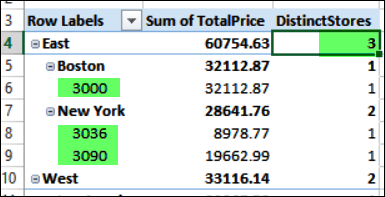
The pivot table screen shot below shows an example of a unique count, in column C.
There are 3 unique stores in the East Region:
- Boston has 1 store – Store 3000
- New York has 2 stores – 3036 and 3090.
In column C, you can see a count of those unique stores in each region or city

The sections below show how to get that Distinct Count, using one of the 4 different methods.
Video: Count Unique in Excel Pivot Table
In this short video, I show how to count unique items (distinct count) in a Microsoft Excel pivot table. This method works in Excel 2013 and later versions.
This is method 1, in the section below.
1) Easy Steps – Excel 2013 or Later
In Excel 2013 and later, a normal pivot table does not have a Unique count function.
However, when you create a pivot table, there is a check box where you can choose to “Add this data to the Data Model”
- If you check that box, Excel creates an OLAP-based pivot table, instead of a normal pivot table
- OLAP-based pivot tables have a Distinct Count function
- Add any value field to the pivot table, then summarize the values with Distinct Count
Detailed steps for this method are on the Pivot Table Unique Count page, on my Contextures site.

2) Pivot the Pivot – Excel 2010 and later
If you’re using Excel 2010 or later, you can use this “Pivot the Pivot” workaround.
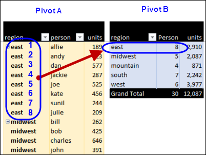
In this method, you’ll create 2 pivot tables:
- Pivot table A summarizes the data, and it is formatted to show the labels in every row
- Pivot table B is based on the worksheet range that contains pivot table A
- you can use a dynamic named range
- or create the named range in a macro, when the data is refreshed
Detailed steps for this method are on the Pivot Table Unique Count page, on my Contextures site.

3) Formula in Source Data – All Versions
If you’re using Excel 2007 or an earlier version, there’s no option for repeating labels in a pivot table.
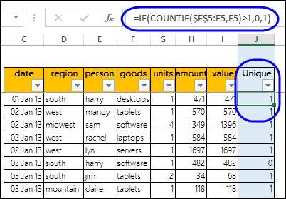
So, instead of the previous method, you can add a formula in the pivot table’s source data, to calculate a unique count.
NOTE: This method slows down the workbook, so use the “pivot the pivot” method if you can, for a large data set.
- In the screen shot below, you can see the COUNTIF formula that’s used in column J.
- It returns a 1 in the first row that a person’s name appears, and a 0 in subsequent rows for that person.
Detailed steps for this method are on the Pivot Table Unique Count page, on my Contextures site.

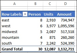
Then, in the pivot table, I did these two steps:
- added the “Unique” field
- changed its pivot table caption to “Person “

4) Power Pivot Distinct Count
If you’re creating a Power Pivot in Excel, instead of a normal pivot table, you’re in luck – it has a DISTINCTCOUNT function.
This video shows how to get a unique count in Excel Pivot Table, with Power Pivot.
Sample File: To follow along with the video, download the sample file that was used for this video
Get Details and Sample File
To learn more about these techniques, go to the Pivot Table Count Unique page for the full details, and download the sample file.
The zipped file is in xlsb format, and contains an optional macro. You can manually refresh the pivot tables, if you prefer.

2013 Excel adds distinct count feature when creating a pivot table. Just put a check on option “add to data model”(or something like that)…no need for Power Pivot.
Jay, thanks for the tip!
Jay,
Thanks so much for the tip.
VJ
Hi,
You end this article saying: “However, this method shows down the workbook, so use the “pivot the pivot” method if you can.”
Did you mean “slows” down or is that supposed to be “shows” down?
If it is “slows” down, what might the reason be for slowing the workbook down? It not an array function, unless you are referring to a very large volume of data.
TX Debra. 🙂
Thanks Rudi, I’ve fixed the typo, and added “for a large set of data”. You can see tables with Roger’s performance measurements in the article:
http://www.contextures.com/pivottablecountunique.html#performance
Why don’t you try just add count formula below or next to pivot? 😉 For example pivot with a region as a columns labels, person as a rows labels, as a value anything(count of persons) and then count formula below pivot(one for each region)?
Is there a way to filter the output of a pivot table where the value of Count of SelectedField is say less than or greater than some value? I know I can do this in a second step. I really want to finished pivot table to have the desired result in the first step.
i.e.
original:
Susan 1
Jack 19
Karen 5
Sam 42
Rick 28
Rebecca 22
with Filter applied
Count of fldName > 10
Jack 19
Sam 42
Rick 28
Rebecca 22