
This step-by-step video shows how to unpivot data in Excel, using Power Query. This creates better source data that you can use to build flexible pivot tables. And it doesn’t change your original data – you can leave that as is!
Video: Unpivot Excel Data with Power Query
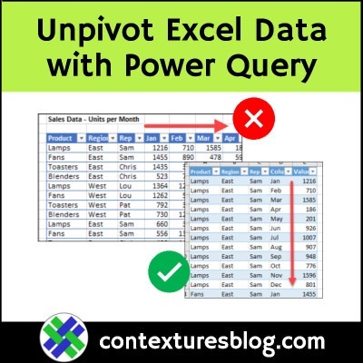
Unpivot your Excel data, if needed, to change it from a horizontal report layout to normalized column layout. You can build better pivot tables from the revised data, and the original data won’t be affected. Win – Win!
In this step-by-step video, I show how to unpivot using Power Query, and there are written steps and a sample file on the Unpivot With Power Query page on my Contextures site.
Tip: For other ways to unpivot Excel data, without Power Query, go to the Fix Pivot Table Source Data page on my Contextures site.
Video Timeline
- 00:00 Introduction
- 00:27 Named Excel Table
- 01:24 Start Power Query
- 02:02 Rename Query
- 02:19 Delete Step
- 02:42 Remove Column
- 02:57 Unpivot Data
- 03:31 Rename Columns
- 03:50 Detect Data Type
- 05:10 Load Data
- 05:41 Refresh Data
- 05:59 Get the Sample File
Why Unpivot Data?
Before you can build a flexible pivot table in Excel, you might need to rearrange your source data.
For example, in the screen shot below, there is a separate column for each month’s sales amounts.
This layout makes it easy to enter data, but the monthly columns cause problems if you need to create pivot tables.

For example, in the screen shot below, you can see a pivot table built from that monthly sales data.
Instead of one pivot field for amounts, there is a separate pivot field for each month’s amounts.
It will be a painful process to get an annual total!

Unpivot the Data
To avoid that pivot table problem, you can “unpivot” the data, to get all the amounts in one column.
The screen shot below shows an example of rearranged data. Now,
- all the sales amounts are in a single column
- all the month names are in a single column
- each row has details for a single product sale
Follow the steps in the video above, to fix your data, if it’s in a horizontal layout.
And, for written steps, you can go to the Unpivot With Power Query page on my Contextures site.

Get the Sample File
To test the Power Query Unpivot technique, you can go to the Unpivot With Power Query page on my Contextures site, and download the Excel sample workbook.
The file is in xlsx format, and is zipped. There are no macros or queries in the file.
____________________________
Unpivot Excel Data with Power Query Step by Step Video

____________________________