Excel Hyperlink to Next Empty Cell

Last week, someone asked me how to make an Excel hyperlink to next empty cell. See how to set that up, in a couple of different situations.

Hyperlink to Next Empty Cell

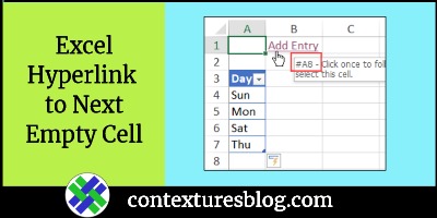
The request was for a cell that said “Add Data”, with a link to the next empty cell in a data entry list.

It wasn’t clear is the list was just on the worksheet, or in a named table, so I made 2 examples.

Next Empty Cell – Named Table

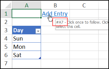
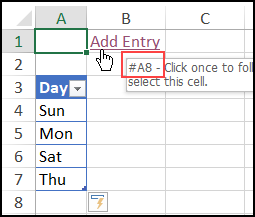
In the first example, the list is formatted as a named Excel table, with the heading in cell D3.

If you point to the hyperlink in cell B1, it shows the address of the next empty cell below the table – cell A7.

HYPERLINK Function – Named Table

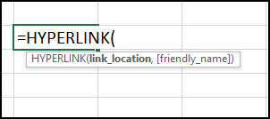
In cell B1, there’s a formula with the HYPERLINK function. The HYPERLINK function has 2 arguments:

1. link_location – where the link should take us
2. friendly_name – text for the hyperlink (optional)

Friendly Name

Let’s look at the easy part of that formula first – the friendly name.

In this example, cell B1 should say, “Add Entry”, so that will be in the 2nd argument.

=HYPERLINK(link_location, “Add Entry”)

NOTE: If you omit the friendly name argument, the cell shows the link location.

Link Location

When you’re linking within an Excel workbook, the link has to start with a number sign – #.

The next empty cell will be somewhere in column A, below the last row in the named table, tblDays.

Here’s the start of the link location argument, with those 2 characters:

=HYPERLINK(“#A”

Empty Cell Row Number

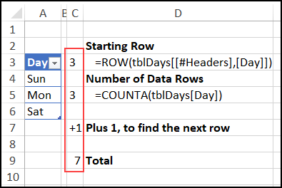
Next, the formula has to calculate the row number for the next empty cell.  That row is the SUM of these 3 numbers:

• The table’s starting row
  • =ROW(tblDays[[#Headers],[Day]])
• The number of data rows in the table
  • =COUNTA(tblDays[Day])
• Plus one, to get to the empty cell below the table

Here’s the formula in cell B1:

=HYPERLINK(“#A” & SUM(COUNTA(tblDays3[Day]), ROW(tblDays3[[#Headers],[Day]]), 1), “Add Entry”)

Test the Hyperlink

To test the hyperlink, try these steps:

• Click the hyperlink to go to cell A7, and type a day name there.
• Then, point to the hyperlink in cell B1 again.

The screen tip now shows A8 as the address that it will go to, as the next empty cell.

HYPERLINK Function – Worksheet

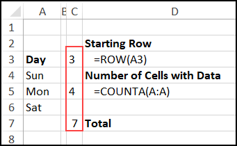
When the list is on a worksheet, instead of a named table, the empty row calculation is different. The rest of the formula is the same.

That row is the SUM of these 2 numbers:

• The list starting row
  • =ROW(A3)
• The number of cells with data in column A
  • =COUNTA(A:A)

Here’s the formula in cell B1:

=HYPERLINK(“#A” & SUM(COUNTA(A:A), ROW(A3), “Add Entry”))

More HYPERLINK Examples

To see more ways to use the HYPERLINK function, watch this short video.

For the written steps and sample file, go to the Hyperlinks page on my Contextures site.

Get the Sample File

There are several sample files on my Excel Hyperlinks page, and the Empty Cell hyperlink example is in the first workbook – General Examples.

_____________________

Excel Hyperlink to Next Empty Cell

_________________________