Drop Down from Filtered Excel List

Someone asked me how to make a data validation drop down that only shows the visible rows from a filtered list. I created a sample file that shows how you can do that, and here are the details on setting up a drop down from filtered Excel list.

Video: Drop Down from Filtered List

Update: Here’s a new video that shows how to set up the drop down from a filtered list, step by step. The written instructions are below the video.

Employee List

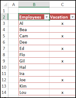
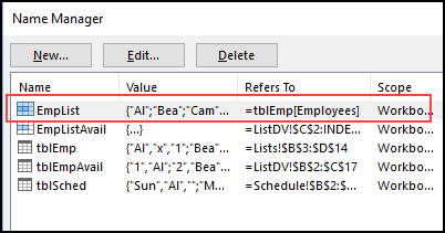
In this example, the workbook has a list of employees, in a formatted Excel table (tblEmp).

There is a named range – EmpList – based on the Employees column in that table.

Simple Drop Down List

If you create a data validation drop down list, it shows all the items from the source list. There are basic instructions for setting up a drop down list on my Contextures website.

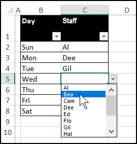
In the sample workbook, there is a schedule sheet, with a drop down list based on the EmpList named range.

Click the arrow in the Staff column, and select any of the employee names.

Filtered List of Names

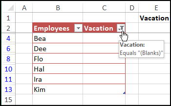
In the Employee table, there is a column to mark an X, for anyone who’s on vacation. To see who’s available for work, you filter the list, and hide all the rows that contain an X in the Vacation column.

That doesn’t affect the data validation drop down list of employees though, on the Schedule sheet.

Even though only 6 names are showing, the drop down list still includes all of the employee names.

Number the Visible Rows

To create an employee list that only includes the visible rows, we’ll add a new column to the Employee table.

The new column has the following formula, using the SUBTOTAL function:

=–SUBTOTAL(3,B$3:B3)

• The function has COUNTA (3) as the first argument
• The range starts at cell B$3 (locked row), and goes down to the current row, B3 (not locked)

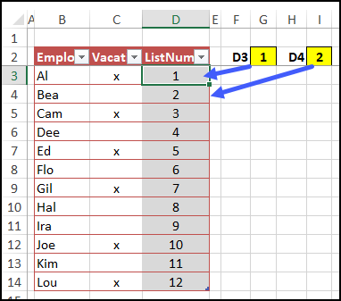
Here is the table with all rows visible, showing the SUBTOTAL formula results in each row. There are cells at the top that link to the first 2 rows, so we can check the results, after some of the rows are hidden.

To learn more about numbering visible rows with SUBTOTAL, read this article, that I wrote a few years ago. It explains why the two minus signs are at the start of the formula.

Apply a Filter to the List

Next, the Employee list is filtered, so hide all the rows marked with an X.

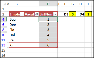
Here is a screen shot of the filtered list, and the visible rows are numbered from 1 to 6.

The SUBTOTAL function ignores rows that have been hidden by a filter, so it will only calculate a count on visible rows

The formulas at the top show that there is a 0 result for the SUBTOTAL function in the hidden row for D3

Create a List of Available Employees

Now that the full list is numbered, we’ll create a second list of employees. The new list will have formulas, to get the names, based on the numbers in each row.

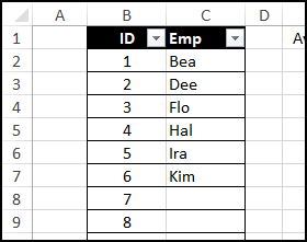
The new list has the headings, ID and Emp, and numbers are typed in the ID column. Be sure to add at least as many numbers as there are employees in the main list – I added a few extra numbers too.

In the Emp column add this formula, to return the employee name, based on the ID numbers.

=IFERROR(INDEX(tblEmp[Employees], MATCH(B2,tblEmp[ListNum],0)),””)

The INDEX function returns a name from the Employees column, for the row that has the same number as the ID.

This screen shot shows the new list, with the numbered names from the filtered main list.

Count the Visible Names

We want to use this short list for our drop down list, so we’ll create a dynamic named range with the names in our new list.

To make the named range the correct size, a formula on the worksheet get the number of visible names.

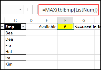
To get the count, the cell contains this MAX formula:

=MAX(tblEmp[ListNum])

That returns the highest number from the main list.

Create a Dynamic Named Range

To create a dynamic named range, that will adjust its number of rows based on the count of visible names, follow these steps:

• On the Ribbon’s Formulas tab, click Define Name
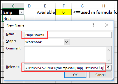
• Type the name: EmpListAvail
• For the Scope, select Workbook
• In the Refers to box, enter this formula:
• =ListDV!$C$2:INDEX(tblEmpAvail[Emp], ListDV!$F$1)
• Click OK

Check the Dynamic Range

To check the Dynamic Range, follow these steps:

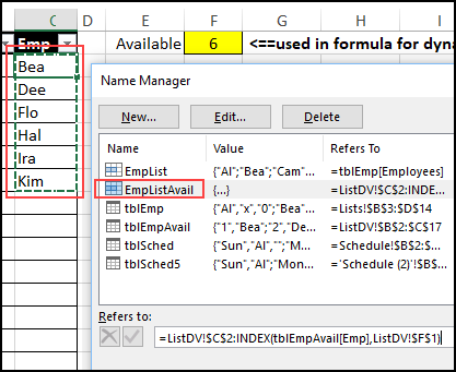
• On the Ribbon’s Formulas tab, click Define Name
• Click on the new name: EmpListAvail
• Click in the Refers to box, and the range will be highlighted on the worksheet, with “marching ants”.
• Click Close.

How the Formula Works

The formula for the dynamic range starts at cell C2 on the ListDV sheet.

• • =ListDV!$C$2:

Then, the INDEX function returns the end cell in the Emp column, based on the number in cell F1

INDEX(tblEmpAvail[Emp], ListDV!$F$1)

If that number changes, the end cell will adjust to the the new number.

Fix the Drop Down List

The final step is to create a drop down list that is based on the dynamic list of employees, instead of the full list of names.

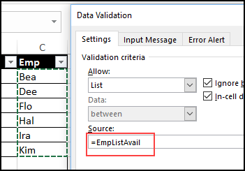
• On the Schedule sheet, select all the cells that have the drop down list for employee names
• On the Data tab of the Ribbon, click Data Validation
• In the Source box, refer to the dynamic named range: =EmpListAvail
• Click OK

Test the Drop Down List

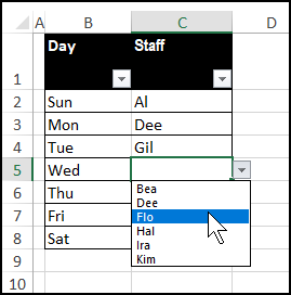
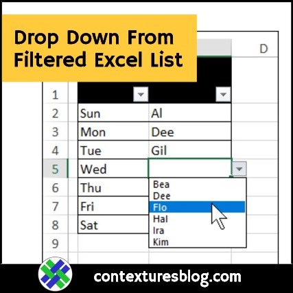
Now, test the drop down list, and it should show the short list of available employees, instead of the full list.

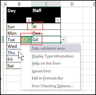
NOTE: Some names might have previously been selected from the full list, like Al and Gil in the screen shot above. Be sure to fix those, or you might see Data Validation error warnings.

Get the Sample File

To get the sample workbook for this blog post, go to the Drop Down From Filtered List page on my Contextures site.
The zipped file is in xlsx format, and does not contain macros.

More Tutorials

Data Validation Basics

Create Simple Dependent Lists

Flexible Dependent Drop Downs

Dependent Drop Downs – Dynamic Arrays

FILTER Function Examples

FILTER Function Reports

________________

Drop Down from Filtered Excel List

________________