Pivot Chart Title from Filter Selection

Instead of adding a static title to your Pivot Chart, use a worksheet formula to create a dynamic chart title. Then, when you make a selection in the Report Filter, the chart title will change too. The video below shows the step-by-step instructions.

Pivot Chart Title

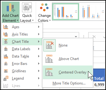
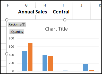
After you create an Excel Pivot Chart, you can add a title at the top, to explain what the chart shows.

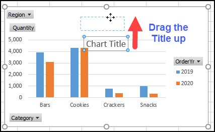
Excel inserts a generic Title, which you can change, move, and format.

Create a Dynamic Title

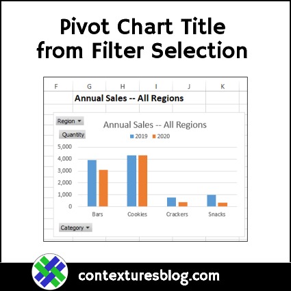
Instead of typing some text in the chart title, you can use a worksheet formula to create a dynamic title.

In this example, the following formula is in cell G1:

=”Annual Sales — ” &
IF(C2=”(All)”, “All Regions”,
IF(C2=”(Multiple Items)”, “Multiple Regions”, C2))

Formula Beginning

The formula result starts with the text string:

“Annual Sales – ” &

The ampersand operator ( & ) joins that string with the text that follows it.

Show the Filter Selection

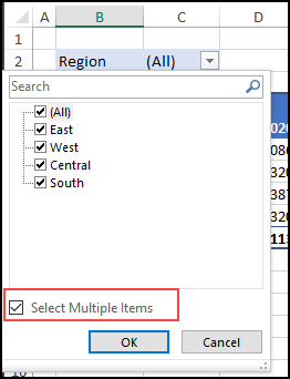
The formula result ending depends on what is selected in the pivot table’s Region filter

IF(C2=”(All)”, “All Regions”,
IF(C2=”(Multiple Items)”, “Multiple Regions”,
C2))

If ALL Regions are selected, the formula ends with “All Regions”
If multiple Regions are selected, the formula ends with “Multiple Regions”
If only one Region is selected, that region’s name, in cell C2, is shown.

Link Chart Title to Formula Cell

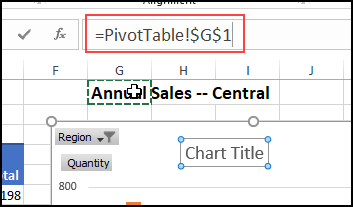
Then, link the Pivot Chart Title to the formula cell, and the Title changes when you select from the Pivot Table Report Filter.

After you create the link, the chart title changes when you make a different selection from the Region filter in the pivot table.

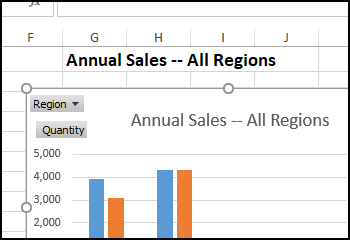
Here is the pivot chart title, after the Region filter is cleared, and data for all the regions is showing.

Video: Get Chart Title from Filter

Watch this video to see how to set up the formula, and link the pivot chart title to the formula cell.

Download the sample file from the Pivot Chart page on my Contextures site, to follow along with the video.

Video Timeline

00:00 Intro
00:19 Add a Pivot Chart
01:14 Add a Chart Title
01:57 Region Filter
03:01 Create a Formula
03:22 Formula Rules
04:02 Start the Formula
06:52 Link Title to Formula Cell
07:51 Get the Sample File

Download the Workbook

Download the sample file from the Pivot Chart page on my Contextures site, to follow along with the video.