If a list contains blank cells, the usual method for creating a dynamic named range doesn’t work. Usually, you would use an OFFSET formula, and count the entries in the column, to calculate the number of rows in the range. Here is a workaround to create a dynamic list with blank cells.
Blank Cells in a Column
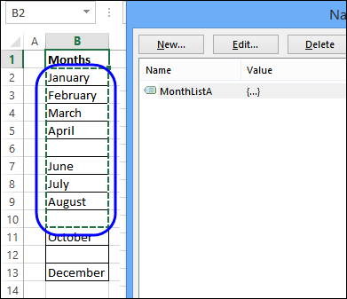
When there are blanks, as in the screen shot below, the dynamic range with blank cells is incorrect. There are 9 items, so 9 rows are included, but the last item is in the 12th row of the list.
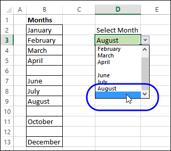
If you create a drop down list based on this dynamic range of 9 rows, it includes blanks, and August is the last month, instead of December.
Fix the Problem
To fix the problem, create a list with all the items, and no blank cells. That will create a usable source list for the drop downs, instead of trying to create a dynamic list with blank cells.
Number the Non-Blank Cells
To create a drop down list without blanks, based on a range with blank cells, add formulas to the worksheet.
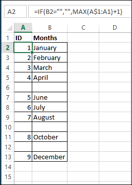
First, add a formula in cell A2, and copy it down to cell A13. This will number the cells that are not blank.
=IF(B2=””,””,MAX(A$1:A1)+1)
Create a List Without Blanks
Next, to create a source list without blanks, use formulas to pull the numbered items into a new column.
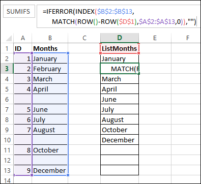
Enter this formula into cell D2, and copy down to D13. This INDEX/MATCH formula creates a list with all the blanks at the end.
=IFERROR(INDEX($B$2:$B$13,MATCH(ROW()-ROW($D$1),$A$2:$A$13,0)),””)
Create a Dynamic Range Without Blanks
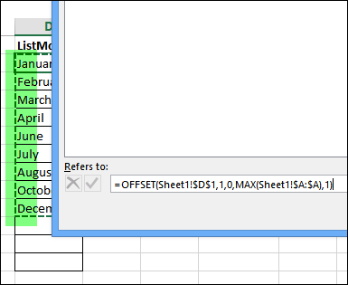
After you use formulas to create a second list, without the blanks, you can name that range, and base the dynamic range on that.
This range is named ListMonths, and uses the MAX from column A as the row count.
=OFFSET(Sheet1!$D$1,1,0,MAX(Sheet1!$A:$A),1)
New Dynamic Range
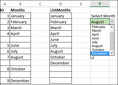
If you create a drop down list based on the ListMonths range, it does not include blanks, and December is the last month.
Instead of the original dynamic list with blank cells, the new list does not have blanks, and can be used for the drop down lists.
Download the Sample File
To see the formulas, you can download the file from my Contextures website.
On the Sample Excel Files page, go to the Data Validation, and look for DV0063 – Dynamic List With Blank Cells. The zipped file is in xlsx format, and does not contain macros.
________________________

Hi Debra
This is a clever solution to a perennial problem, though I do wonder if we as an Excel community too often look for “work arounds” to solve problems by building more and more ‘structure’ into our workbooks, when there are simpler methods. In your example you’ve had to add two additional ranges, whereas a quick and simple sort of the original months table would overcome the problem. I know that there is generally no shortage of spreadsheet real-estate so so space is not an issue, but I believe less (without being austere!) is best.
When I have a number of such tables that need to by dynamic, I use a separate sheet for them, and to cater for further rows being added in future, either:
1. locate the ranges/tables vertically one under another (with a couple of blank rows in between), or more usually
2. arrange the ranges/tables side by side, and build a boundary fence (\=) in a single row below all tables a couple of rows under the longest table range – and anchor the range references for the COUNT or COUNTA function (used in the OFFSET function to return the dynamic range) to this fence. Then I just add new values to each table above the fence as and when required without having to anything more. If one table reaches the fence, I just insert a few more blanks rows across all tables immediately above the fence. I also apply Conditional Formatting to fill cells in the tables with a light yellow colour if blank to indicate that these are available for input.
Cheers
Col
interesting post, Debra, thanks!
I also like Col’s approach as I also tend to avoid creating additional data. I would go with something like “fill’em up with zeros” (or similar) and then conditional format them to not show with “;;;”
Bob Umlas follows a similar approach as you do, Debra, utilizing array formulas and the SMALL function
Hi Debra,
I learned about Data Validation long before. But I have to say it you really take me to the next level of using Data Validation. Thank you so much for all these articles regarding Data Validation. Actually, as inspired by this post and also inquired by a friend, I am going to write a post about making a Dynamic List that always put the man with least hours of job assigned on the top of the list. I will share with you once I am done with the post.
Hi Col and Phil, I agree with you on simplicity. However, something simple to you may not be simple at all to ordinary users in real workplaces. In order to have flexibility, we may have to trade off some extra cells to make the spreadsheet user-friendly.
Hi Debra,
As mentioned, I have finished my post.
http://wmfexcel.wordpress.com/2014/03/07/dynamic-dropdown-least-hours-assigned-always-on-the-top/
Appreciate your comment. 🙂
Hi,
I have data in Column A (Eg: Jan, Mar, Feb, Apr) and how can i get the data in sorting order in drop down.
Wonder if there is a way to put a standard cell first and if i use the drop down, then it will be selected. dunno if that makes sense to anyone.
excel if returning an error stating ‘IFERROR’ is unrecognized text. Not sure how to overcome that.
This feature about drop down list to skip blanks in between is great!.. Will this work to suppress the blank rows at bottom of a range also ? i mean, if data is in Cells B10 to B15 and B16:B20 are blank, the list should not display the latter, but only first 5 items (and no blank rows beyond it).
Thank you Debra!
Exactly what I needed!
You’re welcome Tim! Thanks for letting me know that it helped.
This is a very informative post. Thanks so much! By referring to this, I was able to implement this solution on one of our data forms.
I just have a simple question – if one of the entries in the list needs to be removed, and I ‘delete’ that cell entry and then ‘cut’ the other entries below the deleted entry, paste them one cell up, then the formulas in column ‘ID’ get corrupted (#REF) and the list gets messed up. I believe this is because the formulas in column ID are relative reference.
Is there a way to workaround this?
Your help is much appreciated.
Ryan
Ryan: If you just clear/delete the contents from the cell in the original input list and leave it blank, you need do no more! The second table containing the INDEX/MATCH combo formulae will just have another blank cell to deal with in the same way as they dealt with those that existed before your change.
I came across this article and it was perfect to spark my idea of what to do to fix and issue we had. We needed something that works precisely like this but had to tweak it in the ID “helper” column to not number if the person didn’t have any data for the month. In our case the list wasn’t missing data we just wanted a short list that contained only those who had data. A simple sort would not have worked for us. Hiding the columns would not work because we do not want to confuse all the end users who are not very familiar with excel. Thanks so much for sharing this.
How to EXCLUDE BLANK VERTICAL COLUMNS using ID COLUMN with OFFSET MAX or INDEX MATCH?
How can I use same formula but not count cells with formulas that have no results.
this starts with the formula: =IFERROR(INDEX($B$2:$B$13,MATCH(ROW()ROW($D$1),$A$2:$A$13,0)),””), but what if one doesn’t know the last cell in the range, that is, the “A13” cell? I need this to be dynamic, as my range could be any length, depending on the user’s input. How could this be done?