In a previous article, we combined the MAX and IF functions, to find the highest price for a specific product. Today we’ll use that technique to find the latest date that a product’s price was changed. Then, using the product name and that date, we can find the latest price for specific product – even if it isn’t the highest price.
Product Pricing Table
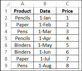
In this example, there is a price list in cells A1:C9. There are three columns: Product, Date and Price.
Find the Latest Date
If we want to find the latest price for Pens, the first step is to figure out the last date that its price was changed. To do that, we’ll use the MAX and IF functions. This is an array function, so you’ll press Ctrl+Shift+Enter, instead of just pressing Enter, after typing the formula.
-
- Enter the product name — Pens — in cell A12.
- To calculate the latest date in cell B12, enter this formula, and press Ctrl + Shift + Enter:
=MAX(IF($A$2:$A$9=A12,$B$2:$B$9))
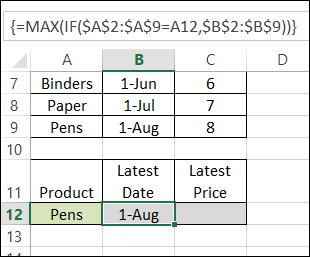
The formula looks for the selected product name in column A — $A$2:$A$9=A12
Then, it finds the highest date for that product in column B — $B$2:$B$9
Calculate the Latest Price
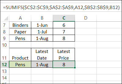
Next, we’ll use a SUMIFS formula to find the latest price for Pens. This formula can be used in Excel 2007, or later versions. If you’re using Excel 2003, you can use SUMPRODUCT – see that example in the next section.
NOTE: This solution assumes that a product’s price is never changed twice on the same date.
Here is the SUMIFS formula, in cell C12:
=SUMIFS($C$2:$C$9,$A$2:$A$9,A12,$B$2:$B$9,B12)
Excel 2003 Formula
The SUMIFS function isn’t available in Excel 2003, so if you’re using that version, you can use the SUMPRODUCT function instead:
=SUMPRODUCT(($A$2:$A$9=A12)*($B$2:$B$9=B12)*($C$2:$C$9))
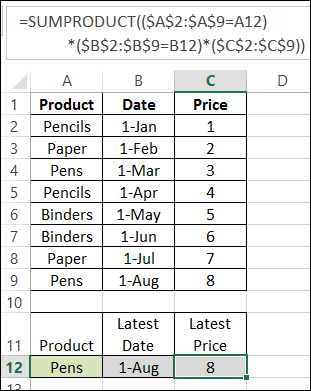
Download the Sample File
You can download the sample file from the MIN and MAX Functions page on my website.
__________________________


Well done, Debra!
I’ve always done stuff like this with formulas as well, but a PivotTable works well too. Just sort the date field newest to oldest, and use a “Top 10” filter to display only the top 1 items.
Great ! This will save the time of writing a macro. Also some users may not like the (slightly) lower security settings that macros require.
Thank’s that technique to find the latest date that a product’s price was changed.
An alternative for the SUMPRODUCT formula in 2003 is using the SUM function as an array formula (with the same arguments as SUMPRODUCT), i.e. the formula is exactly the same except for “PRODUCT” and is entered with Ctrl+Shift+Enter instead of just enter.
I have a problem with Max IF. I need to find the max date combining 2 different columns of 2 different workbooks with criteria. Pls give me a formula.
this is what is expected and I have a problem to update my tables
Table One “Products”
Colomns ” PDate, Item, Price”
1/1/2017 – AAA – 50.00
4/1/2017 – AAA – 65.00
Table one “Invoice”
Colomns “In Date, Item, Qty, Amount”
1/5/2017 – AAA – 15 – Should be 1/1/2017 Price
5/5/2017 – AAA – 10 – Price should be latest Date
Earliest I use vlookup to get prices but now prices are changed So Please help me to keep both prices in the invoice table depend on the invoice date..
Jey, you can use an array formula to find the applicable price for the product, based on the invoice date. I’ve uploaded a sample file on my website:
http://www.contextures.com/excelfiles.html#FN0049
FN0049 – Product Price Based on Date
It really helped me and it works exactly what i needed
It really helped me and it works exactly what i needed, i was searching this for very longer time and spent more time, finally the simple command help me
You’re welcome, Harihara, and thanks for letting me know that it helped you!
Like always great work and I used this on my latest spreadsheet.
What if I want to look up latest price between dates?
Example:
from date = a1
to date = a2
How do I change this formula to include search between these dates?
=IF(G10=0,’PRICE COMPARISSON’!M10,SUMIFS(Table38[[Price]:[Price]],Table38[[Item]:[Item]],Table364894[[RATION ITEM]:[RATION ITEM]],Table38[[Date]:[Date]],G10))
Know it would be a breeze for you
Thank you in Advance
Thanks, Francois, and there’s a date range example here:
https://www.contextures.com/xlFunctions01.html#datesumifs
You could add something similar to your existing formula
Thank you for quick response
Once again the answer lies here somewhere in contextures
Thank you Debra!
Believe it or not
The answer lies right here but I don’t know how to add it with the structured reference in my formula.
=IF(G10=0,’PRICE COMPARISSON’!M10,SUMIFS(Table38[[Price]:[Price]],Table38[[Item]:[Item]],Table364894[[RATION ITEM]:[RATION ITEM]],Table38[[Date]:[Date]],G10))
I Know that this needs to go in formula above
“>=” & $D$2, is the range with the value for criteria 1 (the Start date), and the operator to use with that value (greater than or equal to)
“<=" & $E$2, is the range with the value for criteria 2 (the End date), and the operator to use with that value (less than or equal to)
Try this, Francois:
=IF(G10=0,’PRICE COMPARISSON’!M10,SUMIFS(Table38[[Price]:[Price]],Table38[[Item]:[Item]],Table364894[[RATION ITEM]:[RATION ITEM]],Table38[[Date]:[Date]],”>=” & $D$2,Table38[[Date]:[Date]],”<=" & $E$2))
As always this lady is a genius
Worked for me on that specific formula.
When I tried it on another almost the same formula with array, it says to many arguments.
=IFERROR(MAX(IF(Table3[[Item]:[Item]]=$D11,IF(Table3[[Supplier]:[Supplier]]=G$7,Table3[[Date]:[Date]],”>=” & [03_Monthly_Shopping_Master.xlsm]SL1!$L$4,Table3[[Date]:[Date]],”<=" & [03_Monthly_Shopping_Master.xlsm]SL1!$S$4))),"")
Where did I brake it this time?
Francois, I’m not clear on what your formula is supposed to do. If you take out all the references, this is what remains:
=IFERROR(MAX(IF(Test,IF(Test, if true, if false, extra, extra))),””)
If your version of Excel has MAXIFS, it might do what you need.
https://support.microsoft.com/en-us/office/maxifs-function-dfd611e6-da2c-488a-919b-9b6376b28883