In a pivot table, you can use the built-in Top 10 command, to show the Top 10 or Bottom 3, or almost any other top/bottom summary.
In this post, we’ll see how to show top 3, plus “other”, to show the remaining amounts.
Top 10 Filter Settings
In this screen shot, the Top 10 is selected as a Value Filter.
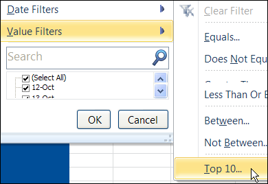
After you select this command, the pivot table shows the selected results, and hides everything else.
Top 3 Plus Other
Recently, I had to make charts that showed the top 3 amounts in a category, and the remaining amounts lumped together as “Other”.
The pivot table summarized the data very efficiently, but wouldn’t create an “Other” grouping.
So, to solve the problem, I used formulas adjacent to the pivot table.
Worksheet Formulas
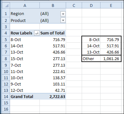
In this example, we want to see the three dates with the highest amounts, and a total for the remaining dates.
The first formula, in column D, pulls the top three dates. An IF formula is used, in case there are fewer than 3 dates in the results. The formula is entered in cell D5, and copied down to cell D7:
=IF(OR(A5=””,A5=”Grand Total”),””,A5)
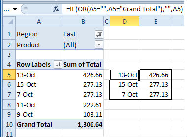
Get Top 3 Amounts
The next formula is entered in cell E5 and copied down to E7:
=IF(D5=””,””,B5)
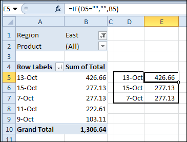
Label Formula for Other Amount
In cell D8, a different formula shows the result of “Other”, if there are 3 or more top amounts.
=IF(OR(A8=””,A8=”Grand Total”),””,”Other”)
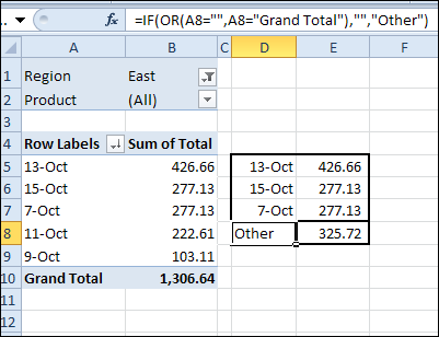
Calculate the Other Amount
In cell E8, the final formula calculates the amount for Other, by subtracting the top 3 amounts from the Grand Total.
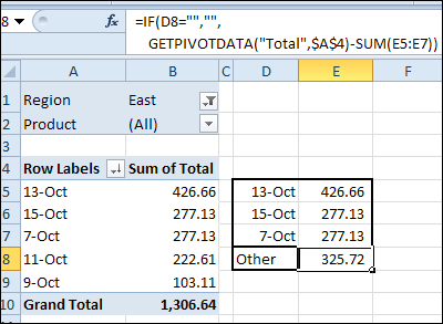
=IF(D8=””,””, GETPIVOTDATA(“Total”,$A$4)-SUM(E5:E7))
Filter the Pivot Table
When you change the pivot table Report Filter selections, the Top 3 and Other amounts change automatically.
Create a Top 3 Chart
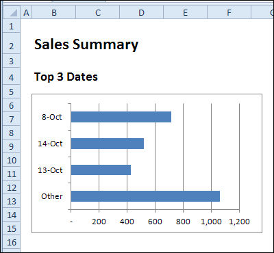
To show the results on an Excel dashboard, you can create a chart, and move it to a Summary sheet.
Add Pivot Slicers
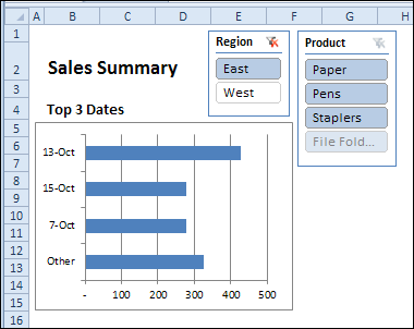
If you’re using Excel 2010, you can add Slicers, so users can change the filter selections, without messing up your pivot table layout.
Download the Sample File
To see the pivot table and all the formulas, you can download the Pivot Table Top 3 Other sample file.
The file is in Excel xlsx format, and is zipped.
There are no macros in the file, and the Slicers are only visible in Excel 2010 or later versions
________________

when I do the total for others it is coming out as #REF!
Hello,
Great article.
What about showing the top 3 most occurring values (text values)?
Say I have a column “Sales” – with a few items – “Bits”,”Bolts”,”Nuts”,”Beer”.
And another column “Dates”.
What I want is to have three cells, showing the top 3 items, based on year.
It would say:
#1 in 2010: Nuts
#2 in 2010: Bolts
#3 in 2010: Beer
Is this possible? Any thoughts?