Make a Valentine Card in Excel

Yes, it’s Valentine’s Day today, and if you were too busy to buy your sweetie a card yesterday, you can make one in Excel. Phew!

Your boss won’t mind if you spend a couple of hours working on this today, because it’s an Excel project! This Excel Valentine card uses a named range, data validation, a formula, and conditional formatting (to change the heart from white to pink to red).

If you won’t have time, or if your drawing skills are worse than mine, you can download the sample Excel Valentine file, at the end of this blog post.

And if you want some romantic music in the background, while you work on your Excel Valentine card, you can listen to the YouTube playlist, compiled by John Walkenbach and his blog readers.

Set Up the Worksheet

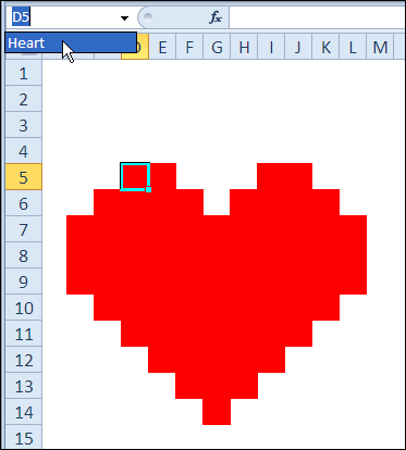
To create the heart shape,

1. Start by making columns A:M narrower, to create square cells
2. Then, add red fill colour to cells in rows 5:14, to create a heart shape
3. Select the coloured cells, and name the range as Heart

Add the Formula

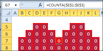
The formula will count how many text items have been added at the top of the worksheet, and the result is used for conditional formatting.

1. Select the Heart range
2. Type the following formula, then press Ctrl+Enter, to enter the formula in all the selected cells:

=COUNTA($E$1:$E$3)

Add Conditional Formatting

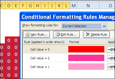
With the Heart range still selected, set up the following conditional formatting:

• =1, light pink fill and font
• =2, dark pink fill and font
• =3, red fill and font

Hide the Heart

The heart shape will be hidden, and only revealed when the Valentine message is selected.

To hide the heart:

1. Select the Heart range
2. Format the cells with white fill and font.

Add the Data Validation Drop Downs

Next, you’ll create three drop downs, for the Valentine message at the top of the worksheet.

To prepare the cells for the drop down lists:

1. Merge cells E1:I1, E2:I2, E3:I3 (yes, merging can cause problems, but it’s allowed on Valentine’s Day)
   • Tip: After you merge E1:I1, drag the Fill Handle, to copy the formatting down to the next two rows.
   • 
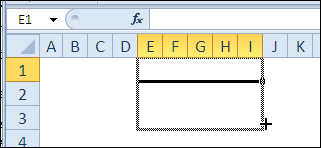
2. Add a bottom border to each merged cell, with red or dark pink border colour.

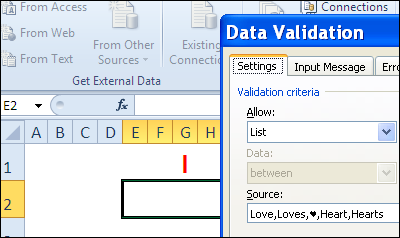
Create the following data validation drop down lists:

• E1: I, You, Everyone
• E2: Love, Loves, ?, Heart, Hearts
• E3: You, Me, Excel

Tip: To type a heart shape, press Alt and type a 3 on the number keypad (if no number keypad, try Fn+Alt+L). On a Mac, another key combination might be needed.

Use the Excel Valentine

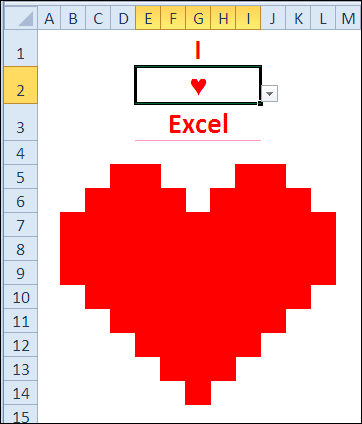
The Excel Valentine heart has white fill and white font, so it’s not visible.
To see the heart:

1. Select one item from the drop down lists, to colour the valentine light pink
2. Select two items from the drop down lists, to colour the valentine dark pink
3. Select three items from the drop down lists, to colour the valentine red

Download the Excel Valentine Card

To see how the card works, you can download the Excel Valentine Card sample file.

The file is in Excel 2007 format, and zipped, and it contains no macros.
_____________