![]() Yesterday, in the 30XL30D challenge, we changed text strings with the REPLACE function, and learned that it can insert characters too.
Yesterday, in the 30XL30D challenge, we changed text strings with the REPLACE function, and learned that it can insert characters too.
OFFSET function
For day 26 in the challenge, we’ll examine the OFFSET function. From a starting reference, it returns another reference, of a specified size, and offset by a set number of rows and columns.
So, let’s take a look at the OFFSET information and examples, and if you have other tips or examples, please share them in the comments.
Function 26: OFFSET
The OFFSET function returns a reference offset from a given reference.
How Could You Use OFFSET?
The OFFSET function can return a reference to a range, and be combined with other functions. Use it to:
- Find sales amount for selected month
- Sum the selected month’s sales
- Create a dynamic range based on count
- Sum the last n month’s sales
OFFSET Syntax
The OFFSET function has the following syntax:
- OFFSET(reference,rows,cols,height,width)
- reference is a cell or range of adjacent cells.
- rows can be positive (below starting reference) or negative (above starting reference)
- cols can be positive (right of starting reference) or negative (left of starting reference)
- height must be positive, and is number of rows in returned reference
- width must be positive, and is number of columns in returned reference
- if height or width are omitted, starting reference size is used
OFFSET Traps
The OFFSET function is volatile, so it could slow down a workbook if used in too many cells. Instead, you could use another function, like INDEX, to return a reference.
Example 1: Find sales amount for selected month
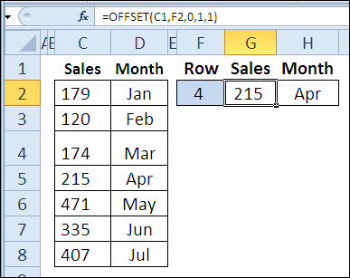
With the OFFSET function, you can return a reference to a range, based on a starting reference. In this example, we want the sales amount in cell G2:
- starting reference is cell C1
- number of rows to offset is entered in cell F2
- sales amount is in column C, so the number of columns to offset is zero
- height is 1 row
- width is 1 column
=OFFSET(C1,F2,0,1,1)
In cell H2, there is a similar OFFSET formula, to return the month name. The only difference is the column offset — 1 instead of zero.
=OFFSET(C1,F2,1,1,1)
Note: The height and width arguments could be omitted, because we want a reference that is the same size as the starting reference. I used them in this example, to show how all the arguments work.
Example 2: Sum the selected month’s sales
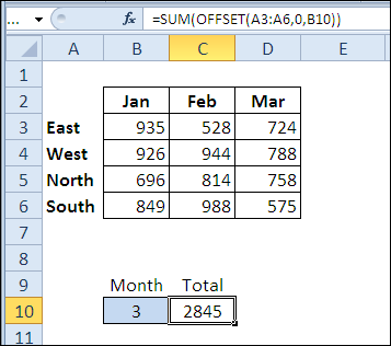
In this example, the OFFSET function returns a reference to the sales amounts for the selected month, and the SUM function returns the total for that range.
In cell B10, the selected month number is 3, so the result is the total of the March sales.
- starting reference is A3:A6
- rows to offset is zero (you could omit the zero, for the same result)
- columns to offset is entered in cell B10
- height and width are omitted, because the reference should be the same size as the starting reference
=SUM(OFFSET(A3:A6,0,B10))
Example 3: Create a dynamic range based on count
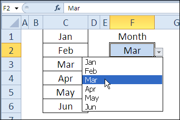
You can also use the OFFSET function to create a dynamic range. In this example, I’ve created a name, MonthsList, with this formula:
=OFFSET(‘Ex03’!$C$1,0,0,COUNTA(‘Ex03’!$C:$C),1)
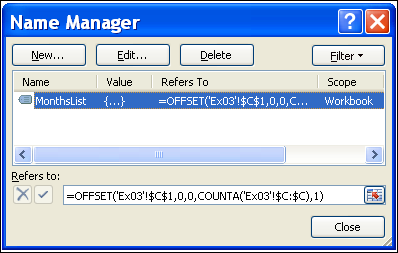
If another month is added to the list in column C, it will automatically appear in the data validation drop down list in cell F2, which uses MonthsList as its source.
Example 4: Sum the last n month’s sales
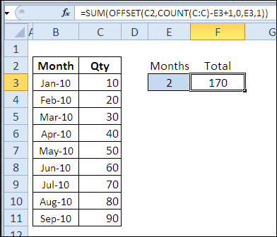
In this final example, OFFSET is combined with SUM and COUNT, to show the total for the last n months. As new quantities are added, the formula result will automatically adjust to include the latest months.
In cell E2, the number of months is 2, so the August and September amounts are summed.
- starting reference is cell C2
- number of rows to offset is calculated by counting numbers in column C, subtracting number in cell E3, adding 1
- quantity is in column C, so the number of columns to offset is zero
- height is entered in cell E3
- width is 1 column
=SUM(OFFSET(C2,COUNT(C:C)-E3+1,0,E3,1))
Download the OFFSET Function File
To see the formulas used in today’s examples, you can download the OFFSET function sample workbook. The file is zipped, and is in Excel 2007 file format.
Watch the OFFSET Video
To see a demonstration of the examples in the OFFSET function sample workbook, you can watch this short Excel video tutorial.
_____________

Deb,
Thanks so much for the 30 in 30 posts. Your succinct tips are very clear and helpful and have shed light on some functions that we a complete mystery to me.
Thanks again,
P.J.
P.J., thanks, I’m glad you’re finding the series helpful. It’s been an education for me too!
I love the OFFSET function. Using it can help you do all sorts of matrix math, which, when used in creating named regions, can be helpful in charting or calculations without having to have thousands of data points.
For example, a named region called OneToN =ROW(OFFSET(Sheet1$A$1, 0, 0, n, 1)) creates an array list of 1 to n. If you need an array of 1’s that is n long then you could call that N1s = MIN(1, OneToN). If you wanted the sum of every other value in a list, then you’d need a list of 1’s and 0’s to multiply your list by before summing and would use OnesAndZeroes = MOD(OneToN, 2), and that sum would be =SUM(OnesAndZeroes * YourList). Oh, and that’s an array function, so you’d need to do ctrl-alt-return to make it work (and get the curly braces in place). The list of things you can do when you understand this wonderful little function are practically limitless…
Sorry. Previous attempt to post had a typo in my email address.
Great article. I love the OFFSET function for creating dynamic named functions in Name Manager for all sorts of things including charts, and I never cease to be amazed at the creative things I see people do with this function in combination with others.
Of note: M-Soft documentation states that the row height and column height arguments must be positive.
That’s not true. Some dynamic ranges wouldn’t work without using negative numbers. Try some negatives to demonstrate.
For a good application of this see “Chart the Last 12 Months Dynamically” here:
http://peltiertech.com/Excel/Charts/DynamicLast12.html
Hope this is of some help to someone.