30 Excel Functions in 30 Days: 10 – HLOOKUP

For day 10 in the 30XL30D challenge, we’ll examine the HLOOKUP function. Not too surprisingly, this Microsoft Excel function is very similar to VLOOKUP, and works with items that are in a Horizontal list.

Less Popular Than VLOOKUP

Poor HLOOKUP isn’t as popular as its sibling, VLOOKUP,  though, because most tables are set up with the lookup values listed vertically.

When was the last time that you wanted to do a horizontal lookup?

Do you ever need to search for a value horizontally, across a row, and then return a value from that column, in a specific row below?

Anyway, let’s give HLOOKUP its moment in the spotlight, and take a look at its information and examples.

Remember, if you have other tips or examples, please share them in the comments.

Function 10: HLOOKUP

The HLOOKUP function looks for a value horizontally, in the first row of a table, and then it returns another value from a different row, in the same column, in that table.

How Could You Use HLOOKUP?

The HLOOKUP function can either find exact matches in the lookup row, or it can find the closest match. For example, an HLOOKUP formula can:

• Find the sales total in a selected region
• Find rate in effect on selected date

HLOOKUP Syntax

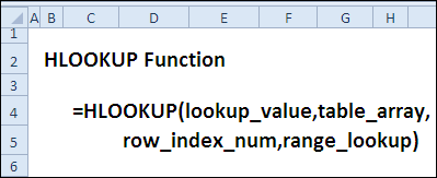
The HLOOKUP function has the following syntax (sequence of arguments):

• HLOOKUP(lookup_value,table_array,row_index_num,range_lookup)
  • lookup_value: the value that you want to look for in the first row of the lookup range — it can either be a value, or a cell reference.
  • table_array: the lookup table — this can be a range reference or a range name, with 2 or more columns in the range. Be sure that the lookup values are in the top row or a table.
  • row_index_num: the row that has the value you want returned, based on the row number within the table. NOTE: This can be different from the worksheetrow number.
  • [range_lookup]: for an exact match, use FALSE or 0 in this argument; for an approximate match, use TRUE or 1, with the lookup value row sorted horizontally, in ascending order.

HLOOKUP Traps

Like VLOOKUP, the HLOOKUP function can be slow, especially if you are doing a text string match, in an unsorted table, where an exact match is requested.

Wherever possible, use a table that is sorted by the first row, in ascending order, and use an approximate match, instead of an exact match.

Tip: You can use MATCH or COUNTIF to check for the value first, to make sure it is in the table’s first row. This can make the calculation much faster in some situations.

HLOOKUP Alternatives

Other Excel functions, such as INDEX and MATCH, can be used to return values from a table, instead of HLOOKUP, and those functions are more efficient.

We will look at the INDEX and MATCH functions later in the 30 Day challenge, and you will see examples of how flexible and powerful those functions are.

Tip: See examples for INDEX and MATCH on my Contextures site: INDEX and MATCH Functions

Also, see these pages on my site, for examples of related lookup functions:

Compare Lookup Functions

VLOOKUP Function

Example 1: Find the Sales for a Selected Region

The HLOOKUP function always looks for a value in the top row of the lookup table.

In this example, we will find the sales total for a selected region — East, West, North or South. Those region names are in the first row of the lookup range, and they are NOT sorted in ascending order.

For our financial report, it is important to get the correct sales amount as our formula result, so the following settings the HLOOKUP function will find an exact match.

Worksheet Setup – Example 1

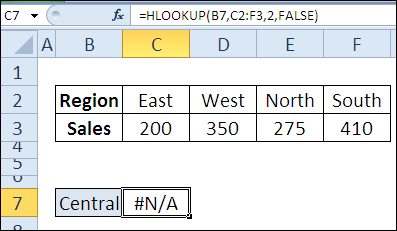
Here are the details on the Excel worksheet setup for this example. You can see the worksheet in the screen shot below:

• a region name is entered in cell B7
• the region lookup table has two rows, and is in range C2:F3
• sales total is in row 2 of the table.
• FALSE is used in the last argument, to find an exact match for the lookup value.

The HLOOKUP Formula

The formula in cell C7 is:

• =HLOOKUP(B7,C2:F3,2,FALSE)

HLOOKUP Error Result

Sometimes, you might get an error resulet with an HLOOKUP formula, as you can see in the screen shot below.

In this case, the region name, “Central”, was not found in the first row of the lookup table, so the HLOOKUP formula result is an error value —  #N/A

Example 2: Find Rate for Selected Date

In most cases, an exact match is required when using the HLOOKUP function,  but sometimes an approximate match works better.

For example, if rates change at the start of each quarter, only those quarterly dates are entered as column headings. It would not be practical to enter every single date in the heading row!

Instead of trying to find an exact match for the date, with HLOOKUP and an approximate match, you can find the rate that went into effect on the closest date.

Worksheet Setup Notes

Here are the details on the worksheet setup for Example 2. You can see the worksheet in the screen shot below:

In this example:

• a date is entered in cell C5
• the rate lookup table has two rows, and is in range C2:F3
• the lookup table is sorted by the Date row, in ascending order
• dates are in the top row of a table
• rate is in row 2 of the table.
• TRUE is used in the last argument, so HLOOKUP will find an approximate match for the lookup value.

HLOOKUP Formula Example 2

The formula in cell D5 is:

• =HLOOKUP(C5,C2:F3,2,TRUE)

How Approximate Match Works

Here is how the approximate match works, in this example:

• If the exact lookup date is not found in the first row of the table, so the HLOOKUP formula finds the next largest value that is less than lookup_value.
• The lookup value in this example is March 15th.
• That value is not in the date row, so the HLOOKUP function returns the rate for January 1st (0.25).
• January 1st is the largest date in the heading row, that is LESS than the lookup date of March 15th

More HLOOKUP Examples

For more HLOOKUP examples, and for tips on fixing HLOOKUP formula problems, go to this page on my Contextures site:

How to Use Excel HLOOKUP Function and Fix Problems

On that page, you’ll see how to:

• use HLOOKUP with the COUNTIF function, for faster calculations
• create an HLOOKUP formula for 2 criteria
• interpret any HLOOKUP error results – #VALUE! and #REF! and #N/A
• fix problems when looking up dates or numbers
• and much more!

Download the HLOOKUP Function File

To see both of the formulas used in today’s 30 Functions in 30 Days challenge examples, you can download the HLOOKUP function sample workbook.

The file is zipped, and is in Excel’s xlsx file format. The workbook does not contain any macros.

Tip: Use this workbook to follow along with the HLOOKUP video, in the next section.

Watch the HLOOKUP Video

To see a demonstration of the examples in the HLOOKUP function sample workbook, you can watch this short Excel video tutorial.

_______________________________