When you create a list in Excel, do you start with a column that numbers the rows? I usually create an ID column and type the number, or use a formula to automatically number them.
In the steps below, I’ll show you the simple numbering system. There’s a fancier formula too, if you’d like to see consecutive numbers when the list is filtered.
Count of Visible Records
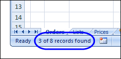
When you use an Excel AutoFilter to filter a list, usually the count of visible records appears in the Status Bar, at the bottom left of the Excel window.
Note: If the Status Bar shows Filter Mode, instead of the record count, you can use one of the workarounds shown here – Status Bar shows Filter Mode.
Record Numbers
That Status Bar count is helpful if you’re looking at the results on the screen. However, it’s not much help if you print the filtered list and give it to someone else.
To make things easier for them, you can add record numbers that will print for each row.
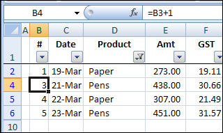
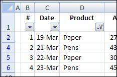
For example, in the screenshot below:
- the visible rows are 2, 4, 5 and 6
- the numbers in column B are 1, 2, 3 and 4.

Add Record Numbers to a Filtered List
In column B of the worksheet list, you could:
- type a list of consecutive numbers
- or, use a simple formula, such as =B2+1
However, those numbers won’t change, if the list is filtered.
For example, in the screenshot below:
- the second record is hidden by the filter:
- the record count, in column B, shows as 1, 3, 4, 5.

Use SUBTOTAL Function
Instead of using the simple formula shown above,you can use a fancier formula, to number the visible rows only.
Here is the revised formula, that I entered in cell B1, using the Excel SUBTOTAL function:
- =SUBTOTAL(2, C$1:C2)
The SUBTOTAL function is designed to ignore rows that are hidden by a filter, so the formula result will change if rows in our list are hidden.
| ⚠️ | Warning: Don’t use this technique if you plan to use Excel’s Subtotal feature (Data>Subtotals) — it may delete your table when you remove the Subtotals. |
Count the Dates
In the sample Excel list, there is always a date in column C, so it’s safe to use the SUBTOTAL function to count the visible dates.
=SUBTOTAL(2, C$1:C2)
1) The first argument in the SUBTOTAL is the number 2. That tells Excel to use the COUNT function in the subtotal result.
- The COUNT function counts numbers and dates only
| 💡 | Tip: If you want to count text entries instead, use 3 as the first argument, and Excel will use the COUNTA function. The COUNTA function counts all types of data. |
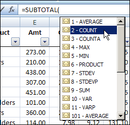
2) The second argument, C$1:C2 is the range of cells that we want to count. Column C contains the dates.
Copy the Formula Down
After you create the formula to number the visible rows in Excel AutoFilter, copy it down to the last row with data.
- The first cell in the range reference, C$1, has an absolute row reference. When you copy the formula down, that part of the formula won’t change.
- The count should always start in row 1.
- The second cell in the range reference, C2, has a relative row reference. When you copy the formula down, that part of the formula WILL change.
- The count should end at the row the formula is in.
With the SUBTOTAL formula, when you apply an Excel AutoFilter, or show all the records, the record numbers in column B will always show a consecutive list of numers..
Problems Hiding the Last Filtered Row
The SUBTOTAL function works well, and renumbers our rows as expected, but there’s something wrong.
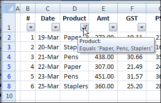
In the screenshot below, the list is filtered to show only two products, as you can see in the AutoFilter pop-up tooltip:
- Paper
- Staplers
However, there is a problem. Can you spot what’s wrong?
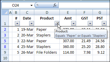
Although the list is filtered for Paper or Staplers, the File Folders record in row 9 is also visible.
Also, its row number button, at the left side of the worksheet, isn’t blue, like the row numbers for rows 2, 3, 5 and 8.
Hidden Named Range
When you use an AutoFilter, Excel creates a hidden named range for the database.
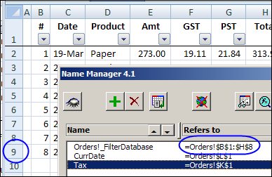
In the screen shot below, I used Jan Karel Pieterse’s Name Manager utility. It lets me see the definition for the hidden name, Orders!_FilterDatabase.
Even though the list ends in row 9, the named range stops at row 8: =Orders!$B$1:$H$8
Why Is Excel Confused?
Why is Excel confused about where the AutoFilter list ends?
If there’s a SUBTOTAL function in the last row of that database, Excel decides that it’s a special row for the list’s totals. The Total Row is not included in the named range.
So, if you want your last row hidden when using the SUBTOTAL function in a filtered list, you can use one of the following workarounds.
Workaround 1: Add a Dummy Row
- [Update] This was my previous workaround. I prefer to use Workaround #2 now.
The first time I ran into this problem, I added a dummy row at the end of the list, with just the SUBTOTAL function, or other dummy data.
Then, that row was treated as the last row, and all the real data is shown or hidden, based on the AutoFilter criteria.
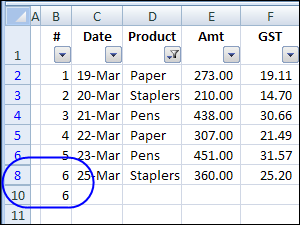
- In the screenshot below, the SUBTOTAL function is copied down to row 10
- When the AutoFilter is applied, row 9 is hidden.
There’s no date in row 10, so it doesn’t affect the record numbering.
Workaround 2: Change SUBTOTAL formula
Recently, I found another workaround, that’s much better than the dummy row solution.
Dick Kusleika was subtotalling filtered rows, and discovered that he could fix the problem by typing two minus signs in front of the SUBTOTAL function.
Note: I left a space between the minus signs below, just for clarity. The formula will work with or without the space.)
=- -SUBTOTAL(2, C$1:C2)
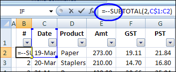
With Dick’s solution, there are two main benefits:
- there’s no need for an extra row, so the worksheet looks better.
- you’ll avoid other potential problems, such as filtering for blanks in one of the fields.
More AutoFilter Tips & Tutorials
AutoFilter Basics
AutoFilter Tips
Advanced Filter Basics
Advanced Filter Criteria
Filter to Different Sheet
Filter Unique Items
Filter with Criteria List
________________

You can also use =Subtotal(2,$C$1:C2)*1 or +0 or – 0 or /1 – Anything along with the Subtotal.
Excel then gets confused and includes the last row inside the filter range
I just want to see the number of the rows (how many of it…)EXCLUDING the hidden ones (with my AUTO FILTER)! it should have been the simplest thing in excel but currently just a TORTURE!it somehow always takes ” the hidden rows” into consideration! No simple solutions in any of the forums! =ROWS(xx:yy) is not working properly
Emre, you can use the SUBTOTAL function: =SUBTOTAL(2,A:A)
There’s an example on the Contextures website Excel AutoFilter Tips page: Count of Filtered Records
This is a great tip.
Another way around the issue noted is to not include the column with the subtotals in the filter range.
Thanks for this tip 😉
thank o lot
Great tip! Thanks a lot!
Great, kind of. I can use the subtotal() approach to find which row I’m on when using filters but now, how do I find the number of the previous or next “visible” row? What I’m looking for is a way to automatically update a difference between rows that are subject to filtering, e.g. a number of days between events.
The argument “2” for Subtotal will ignore rows that are filtered out, but if you hide the rows (vs filtering them out) subtotal will include them. Use argument “102” to ignore hidden rows in a range.
YES! Andres, you are a gem!
This is exactly what I was looking to do, thanks for the tip it was spot on!
Brilliant! Thanks so much
=SUBTOTAL(3,$M$22:M22)
i keep a spread sheet of all the fire extinguishers my company has. I would like to do a count of how many i have inspected this year so far, for quarterly reports. I have filter on location sub location date, etc. What could i use to get the total of FE that i inspected. When i filter the ones i did this year, i want to set up an row that will continually update with the number of FE that i inspect.
I need to number rows in an xls where rows are hidden. I have added a column to the far left where I want the numbering to occur. I tried =(first cell) + 1 and auto fill from there. It worked for the first few rows but then started back at 1 again and I noticed that the auto fill forula for each row is indeed adding 1 to each cell before it. Is there another way?
Great tip. Just want I needed without having to get into VB scripting.
Thanks. It helped a lot.
Exactly what I was looking for, thanks.
Thanks for this explanation about sub totals. I had been tearing my hair out when I realised it was happening to my main spreadsheet. I am actually using =0+SUBTOTAL(9,$J$5:J46), i.e. adding 0 to the subtotal as I find it easier to see than the double negative.
EDIT: Sadly it breaks again as soon as you automatically add a row by pressing tab in the final cell. The next row gets an ordinary sub total, and the filter problem starts all over again. It also mucks up the formatting of teh table so that the rows are not banded. The only way out of it is to remove the sub total from within the table to outside.
i Cant do this! poor me, after doing this, my A2 = 0.
I have a spreadsheet that contains 29,000 line. Excel 2010 will only allow me to view 10,000 – how do I increase this?
when i enter given formula i get error: to few arguments given?
HOW ABOUT SUBTOTAL USING 9 THAT DOESNT WORK IN ADVANCE FILTERING? ANY SOLUTIONS?
=TEXT(SUBTOTAL(2, C$1:C2),0)
using subtotal function
=SUBTOTAL(3,$B2:B$2)
1.CLICK ON THE CELL FOR SERIAL NUMBER
2. PUT ‘+’ OR ‘=’ SIGN
3. SELECT SUBTOTAL FUNCTION
4.SELECT THIRD FUNCTION – COUNTA ( ORDER NO-3)
5. PUT ‘,’
6.SELECT RIGHT SIDE ONE CELL
7. SHIFT + ;
8. PUT $ SIGN AFTER 3, AND IN BETWEEN B&2
My experience..
=subtotal(103,Range)-1+1
the above formula gave me desired results.
Hello everybody,
This worked for me:
=SOUS.TOTAL(103;$A$6:A6)
I wrote this formula in cell B6 because my filtered table visible data starts at row 6.
Then, I dragged down cell B6 until the last cell of column B.
Now, column B contains a list of sequential numbers (1 to 1136) besides column A of filtered data (6 to 2355).
I used the fonction SOUS.TOTAL because my Excel 2016 is in French.
I used the semicolon ; instead of the comma , because the comma didn’t work.
I hope it helps someone.