Filter Pivot Table for Date Range

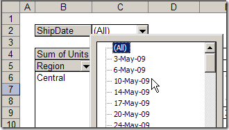
In a pivot table, you might want to see all the orders that were shipped on a specific date.

To do that, you’d move the Ship Date field to the Page area, and select a date from the drop down list.
Filter Pivot Table for Specific Date

Filter for Date Range

Sometimes though, you’d like to show the orders shipped in a date range, instead of just a single date. For example, you might like to show orders with ship dates in the upcoming week, so you can do some planning.

To accomplish this, you could manually hide all the dates in the Ship Date page field, except the dates for next week. However, that might take quite a while if there are lots of dates.

Another option is to add a new field to the source data, to test the ship dates, then add it to the pivot table, as a filter. This might slow things down a bit, if your source data table is very large.

We’ll look at both options in Excel 2003 — the steps are slightly different in Excel 2007.

Manually Hide the Dates

In Excel 2003, there are no check boxes beside the items in a Page field’s drop down list, to allow you to select multiple items.

To hide some of the items in a pivot table’s Page field, temporarily move the field to the Row area, and select the items there, then drag the date field back to the Page area.
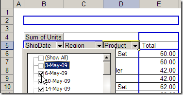
PivotShipDate01a

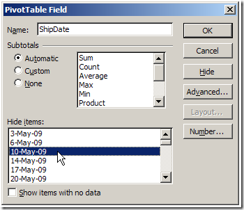
Or, without moving the field in the Page area, you can change the field’s settings.

  1. Double-click on the Ship Date field button.
  2. In the PivotTable Field dialog box, click on dates in the Hide Items list.
  3. Click OK to close the dialog box.

PivotShipDate02

Add a New Field to the Source Data

Manually hiding the dates might work well if you only need to do this occasionally, and the list of dates isn’t too long. Otherwise, the best solution might be to add a column to the pivot table’s source data.

In this case, we’ll add a column named ShipSoon, and use a formula to test if the ship date is within the next 10 days.

  1. In the source data table, add a column with the heading ShipSoon. In this example, the new column is to the right of column A.
  2. In the first data row of the new column, enter a formula that checks the ShipDate in that row. Our first ship date is in cell A2, and the formula will test the date, to see if it’s within 10 days of today’s date.

=AND(A2>TODAY(),A2<=TODAY()+10)
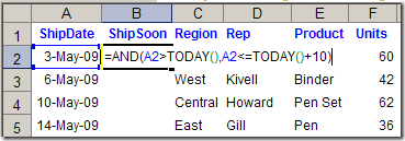
PivotShipDate04a

  • Copy the formula down to the last row of data.

Each row will show TRUE or FALSE as the result of the formula.

Update the Pivot Table

Next, you’ll update the pivot table, and add the new field.

  1. Refresh the pivot table, and add the ShipSoon field to the Page area.
  2. From the ShipSoon Page field dropdown list, select TRUE.
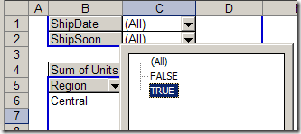
PivotShipDate07a

Refresh the Pivot Table

Remember to refresh the pivot table each day to see the current calculations for the ShipSoon field.

  • To manually refresh the pivot table, right-click on a cell in the pivot table, then click on Refresh Data.
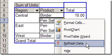
PivotShipDate10a

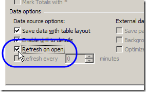
Or, you can set the pivot table to automatically refresh when you open the Excel file.

  1. Right-click on a cell in the pivot table
  2. Click Table Options
  3. In the Data Options section, add a check mark to Refresh on Open
  4. Click OK to close the dialog box.

PivotShipDate11

____________________

Create Excel Pivot Chart With Chart Wizard

If you select a cell in a pivot table and click the Chart Wizard button on the toolbar, a default pivot chart is created, on a new chart sheet.

Sometimes you might want to step through the Chart Wizard, so you can set the options as you create the pivot chart.

Use the Chart Wizard

If you follow the steps below, you can use the Chart Wizard, instead of creating the default pivot chart.

  • Select an empty cell on the worksheet, away from the pivot table and any other data.
  • On the Excel toolbar, click the Chart Wizard button.
  • In Step 1 of the Chart Wizard, select a Chart type and Chart sub-type, then click Next.
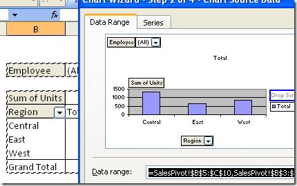
  • In Step 2 of the Chart Wizard, click in the Data range box, and select any cell in the pivot table.
    • The entire pivot table will be automatically selected, and its address will appear in the Data range box.
entire pivot table is automatically selected

Complete Chart Wizard Steps

Next, complete the remaining Chart Wizard steps, selecting the options you want

When you’re done, click the Finish button, to create the pivot chart.

Chart Wizard Note

If you select a pivot table as the data range, you can’t return to Step 2 of the Chart Wizard.

To use a different data range, you’ll have to start over, and create a new chart.
__________________

Rename Excel Pivot Table Value Field

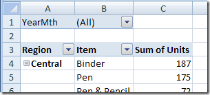
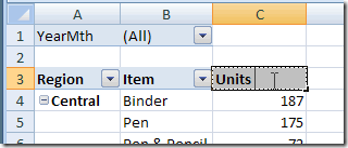
When you add a field to the pivot table Values area, it’s automatically given a custom name, such as Sum of Units.

Default pivot table value field names

Use a Shorter Name

You might want to change the custom name to Units, so it’s easier to read and makes the column narrower.

However, if you select the cell and type Units, you’ll get an error message: “PivotTable field name already exists.”

Use a Slightly Different Name

If you try to create a custom name that’s the same as a field name in the source data, you’ll see the error message. In this example, because one of the fields in the source data is named Units, you can’t use Units as a custom name in the pivot table.

However, you can avoid this problem, by adding a space character to the end of the custom name, and it will be accepted.

PivotUnitsChange

Use Replace All

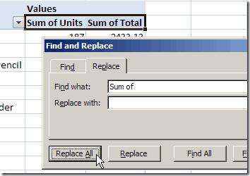
Or, if you have multiple value fields in the pivot table, select all the captions, and use the Replace All command to fix all the captions at once.

  1. In the Find What box, type “Sum of” (do NOTadd a space at the end)
  2. Leave the Replace With box empty
  3. Click Replace All.

This will leave a space at the start of the caption, so it’s different from the original field name, and will be accepted.

Find and Replace dialog box

____________________

Filter Pivot Table Source Data in Excel

When you’re analyzing data in an Excel pivot table, you might want to see the detail behind one of the numbers.

To extract the data, you can double-click a data cell and a new worksheet is created, with the related records.

This is a nice feature, but you’ll end up with extra sheets in your workbook, and will need to clean things up occasionally.

Filter the Source Data

If the pivot table source data is in the same workbook, you can use the following macro, written by Héctor Miguel Orozco Díaz. It filters the source data, based on the pivot items connected to the double-clicked cell.

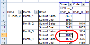
For example, if you double-click the cell circled in screenshot below:

pivotfilter01

the source data is filtered for Class_A, Month_3, Store_1, Code_A cost.

This lets you focus on the detail records, without creating new worksheets.

filtered source data for pivot table

Download the Sample File

Héctor’s code is shown on my Contextures site, and you can download the sample file to filter a pivot table’s source data.

There is also a sample file with a shorter version of the code.
________________

Change Blank Labels in a Pivot Table

In a pivot table, you might have a few row labels or column labels that contain the text “(blank)”. This happens if data is missing in the source data. For example, in the source data, there might be a few sales orders that don’t have a Store number entered.

Continue reading “Change Blank Labels in a Pivot Table”