
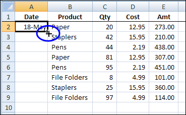
If you’re entering dates on an Excel worksheet, you don’t have to enter each date individually. Just enter the first date, in the top cell. Then, if there is data in the next column, you can use the Fill handle to quickly enter the rest of the dates. See how to AutoFill Excel dates in series or same date, with just a couple of clicks.
Continue reading “AutoFill Excel Dates in Series or Same Date”
Category: Excel Shortcuts
Excel Keyboard Shortcuts for Ribbon
While trying to type a hyphen in Excel 2007, I stumbled onto a handy keyboard shortcut.
I had a bit of an overreach on the hyphen, and hit the F10 key instead. To my amazement, the Ribbon filled with little tags.

Maybe I’ve been living under a rock, but I don’t remember seeing those tiny tags before. Have you noticed them?
There’s a number or letter on each Ribbon tab, like H for Home, N for the Insert tab, and R for the Review tab.
Above that, there is a tag for each icon on the Quick Access Toolbar (QAT) too! They are numbered from 1 to 9, and then a set of descending numbers, from 09 down to 01.
Use the Shortcut keys
Here’s how you can use the shortcut keys that those tags represent:
- First, press the F10 key, to activate the Ribbon.
- Next, type the letter(s) or number(s) that you see on any Ribbon tab or on any of the QAT commands
See Data Tab Commands
For example, I can type an A to activate the Data tab. (Note: Even if the Data tab is active, you’ll have to type an A to see its command tags.)
Tags will appear on the available Data commands.

Because the active cell is in a named Excel table on my worksheet, most of the Data tab commands are available.
- For example, I can type the letter T, to add an AutoFilter
- Or, I could type the letter Q, to start an Advanced Filter.
Useful Feature
It seems like a useful feature, and the only shortcut that I have to memorize is the F10 key.
Anyway, it’s nice to know that a typo can lead to an interesting discovery.
_____________________
Show Excel Formulas Instead of Results
When you’re troubleshooting an Excel worksheet, it may help to see the formulas temporarily, instead of the results. With the formulas visible, you can quickly check that the cell references are correct and the formulas are consistent.

Tip: The keyboard shortcut to show or hide the formulas is Ctrl + ‘ (accent grave, may be above the Tab key on the keyboard).
To view the formulas in Excel 2003:
- On the Tools menu, click Options
- On the View tab, under Windows Options, add a check mark to Formulas.

To view the formulas in Excel 2007:
- On the Ribbon, click the Formulas tab.
- In the Formula Auditing Group, click Show Formulas.

___________________
Create an Excel Chart with One Keystroke
Did you know that it only takes one keystroke to create a chart from data in Excel? Here are the simple steps to create a very quick Excel chart.
- First, select a cell that contains the chart data, or select a heading in one of the data rows or columns
In the screen shot below, the data is in A1:D3, and cell B3 is selected.
NOTE: Cell A1, at the top left corner of the chart data is empty. That makes it easier for Excel to create a quick chart.
- Next, on the keyboard, press the F11 key
A chart sheet is inserted in the active workbook, with a chart in the default chart type, as shown below.
In the sample workbook, the default chart type is a Clustered Column. There are two columns for each month, with East in light purple, and West in dart purple..
Just remember — this is a super quick way to add a chart in Excel. After you insert that Excel chart so quickly, don’t be tempted to spend another couple of hours playing with the formatting, to make it look perfect!
More Excel Charts
_________