
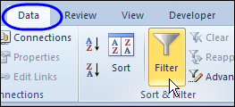
When you turn on the filter in an Excel worksheet list, or if you create a named Excel table, each cell in the heading row automatically shows a drop down arrow. If you don’t need them, here’s how you can hide arrows in Excel AutoFilter.
Category: Excel Filter
Add Products to Excel Order Form
 The summer is off to a good start here in Canada – we had perfect weather for our first long weekend of the season. My garden is almost ready, and I haven’t killed any of the plants yet!
Over the weekend, my Contextures website and blog were moved to a different web host and servers. It seems to have gone smoothly, but please let me know if you see anything strange. Well, stranger than usual. 😉
Click to Add Products to an Order
As you know, when you’re moving, you sometimes find interesting things in the back of the closet. While I was checking the website, I found this sample file, that lets you click to add products to an Excel order form.
On the Data Entry sheet, you can select a product category, from the drop down list.

When a category is selected, the Excel Worksheet_Change event code runs, and lists all the products in the selected category.
Worksheet Change VBA Code
The code uses an Advanced Filter to copy the products onto the Data Entry sheet.

In the list of products, click on any row, in column G, to add that product to the order form.

The Order Form Move Code
Another event code runs when you click on a cell in column G – the SelectionChange event.
It checks the column and row number of the cell that was selected, and checks for an entry in column A.

If the selection was in column G and the row number is greater than 6, and there is something in column A, an X is added to the cell.
Then, the MoveRow code runs, and it copies the selected row to the order form, in the row below the previous product ordered.

Here is the OrderForm sheet, with condiments and dairy products listed.

Future Enhancements to the Product List Order Code
When you go back an look at an Excel project, you can usually think of several things that would improve it. In this example, I’d like to add code that prints the completed order form, and clears the OrderForm sheet.
Is there anything else that you’d add or change?
Download the Product List Order Workbook
To download the product list order form workbook, you can visit the Sample Files page on the Contextures website. In the Filters section, look for FL0016 – Move Items to Order Form.
The file is in Excel 2003 format, and zipped. It contains macros, so enable those, if you want to test the code.
_________________
Drill to Detail With Excel Slicer Filters
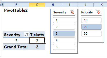
With Slicers in Excel 2010, you can easily filter several pivot tables with a single click. In the screen shot below, the Slicers are filtering the Severity and Priority fields in the pivot table.
However, there is a problem with Drill to Detail with Excel Slicer Filters, in some version.
Continue reading “Drill to Detail With Excel Slicer Filters”
Excel AutoFilter by Typing Criteria
Someone emailed me for help with an Excel AutoFilter last week. He wanted to type the criteria onto a worksheet, and have the filtered results shown automatically.
There are some built-in options for filtering by text, and keep reading to see a worksheet version that Roger Govier designed.
AutoFilter Search in Excel 2010
There is a new feature in Excel 2010 that provides easy searching, though not on the worksheet. You can see an example here, for the Excel 2010 AutoFilter search feature.

AutoFilter Search in Earlier Versions
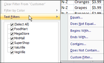
In earlier versions of Excel, you can filter for text, but it’s a bit more work. In Excel 2007 you can use a text filter, which opens the Custom AutoFilter dialog box

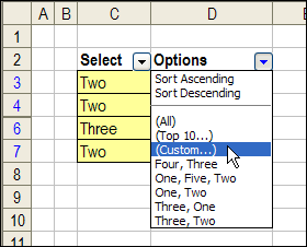
In Excel 2003, use the Custom option on the AutoFilter drop down.

Roger Govier’s FastFilter
If you’d like to enter the AutoFilter criteria on the worksheet, instead of a search box or dialog box, you can use Roger Govier’s FastFilter sample Excel file.
He has set up a table on the worksheet, with an empty row above the table. In that row, you can type one or more criteria, and when you press the Enter key, the table is automatically filtered.
For a simple filter, type an exact match for a value, and press Enter. In the screen shot below, the table is showing only the items from category 2.

You can also use operators, and in the next screen shot I’ve added a “>20” criterion in the Unit Price column.

Use WildCard Characters
If you’re trying to find a specific string of characters in a column, you can use the * and ? wildcard characters. In the next screen shot, I used *b* in the product name column, to find any products that have a “b” somewhere in the name.

Use Multiple Criteria in a Column
You can use special characters for OR (^^) and AND (^), to combine multiple criteria in a single heading cell. In the Category ID column, I used the ^^ characters to find category 2 OR 4. In the Unit Price column, the ^ character limits the price to >20 AND <35.

Remove the Criteria
To clear the filter from a column, just click on the criteria cell, and press the Delete key on your keyboard. If you want to clear all the filters, select all the criteria cells, and press Delete.
Download the Sample File
To download the sample file, you can visit Roger’s Sample Files page on the Contextures website. In the Filters section, look for FL0001 – Fast Filter. There is a download link for the FastFilter zipped file.
The file is in Excel 2003 format, and will work in later versions too. After you open the file, enable macros, so you can test the automatic filter feature.
____________
Excel Filter Macro: Shark Week
It’s hard to believe that Excel Advanced Filter Week is almost over. I hope that the three filter-feeding shark species, and you, have enjoyed this tribute to Discovery Channel’s Shark Week.
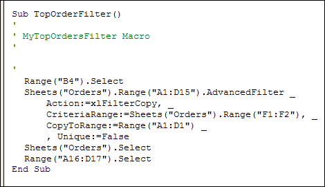
Today, we’ll see how to record a macro while using the Advanced Filter, and edit that macro, so it automatically adjusts if the data changes.
Excel Filter for List Items: Shark Week
On Monday, we declared this Excel Advanced Filter Week, in honour of the three filter feeding shark species. Who said Excel wasn’t exciting?
Excel Filter for Blanks: Shark Week
 Last year, we celebrated the Discovery Channel’s Shark Week, by using the LARGE and FLOOR functions.
This year, we’ll pay tribute to the three known species of sharks that are filter feeders, by declaring this Excel Advanced Filter Week.
Yes, we’ll have three fun-filled, action-packed days of Excel filtering fabulousness – one day for each filter feeding shark. Please hold your applause until all three articles have been posted.
Advanced Filter Criteria Range
We’ll kick off the week’s celebrations by filtering rows with missing data (blank cells) to a different worksheet.
When you’re using an Advanced Filter, usually you would enter a heading, and one or more criteria, in a criteria range, like the one shown below.
In this example, you would be filtering the customer order list for any orders with Cookies as the product.

Blank Cells in Data
However, if you want to filter orders with a blank cell for Product, you can’t just leave the criteria range blank.
A blank criteria cell is interpreted as “No criteria”, so all the records would pass through the filter. That might be fine for a shark, but not for an Excel report.

Filter for Blanks in Advanced Filter
Instead of leaving the criteria cell blank, you can use a formula, to check for empty cells. In this example, the first product data is in cell C2, so the formula is:
=C2=””
The two double quote marks represent an empty string, so if C2 is not blank, the formula result is FALSE.
Only the records that calculate to TRUE would pass through the filter.

Remove the Criteria Range Heading
If you’re using a formula in an Advanced Filter criteria range, the heading can’t match any of the source data headings.
You can either clear the heading cell in the criteria range, or type a different heading.
I usually clear the heading cell, because that’s quick and easy!

Run the Advanced Filter
After you set up the criteria range, you can run the Advanced Filter. Remember, if you want the results on a different worksheet, select that destination sheet before you run the filter.
In this example, the filter is started from the Blank Orders sheet, and the list and criteria range are on the Orders sheet.

Download the Advanced Filter Blanks Workbook
To see the sample data, and test the filter, you can download the Advanced Filter for Blanks sample workbook. The file is in Excel 2007 format, and is zipped.
Watch the Advanced Filter for Blanks Video
To see the steps for setting up the criteria range, and running the filter, you can watch this short Excel video tutorial.
___________________
AutoFilter For Multiple Selections
With data validation and some programming, you can select multiple items from a drop down list, and show the selections in a single cell.
Excel Function Friday: Subtotal and Sumproduct with Filter
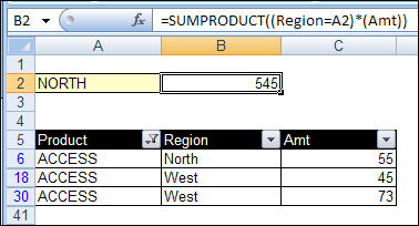
Last week, we used the Excel SUBTOTAL function to sum items in a filtered list, while ignoring the hidden rows. Now we’ll look at ways to use Subtotal and SumProduct with filter settings applied.
Continue reading “Excel Function Friday: Subtotal and Sumproduct with Filter”
Excel AutoFilter or Advanced Filter?
Do you ever use the Excel Advanced Filter feature? Or is all your filtering done with an AutoFilter?