
With Excel’s data validation, you can show a drop down list of items in a cell. You can even create “dependent” drop downs. For example, select a region, and see only the customers in that region. See how to show a warning in Excel drop down list, if the source data is not set up correctly.
Dependent Drop Down Lists
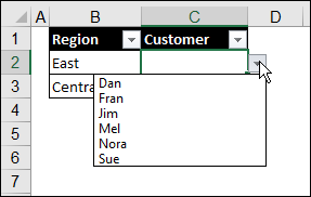
In this example, select a region name in column B. Then, when you click the drop down arrow in column C, the list just shows the customers in that region.
There are a couple of benefits to dependent drop down lists:
- It’s easier to pick a customer from a short list, instead of the full list
- It encourages valid customer entries. (Data validation isn’t bulletproof – there are ways to get around it)
Get the sample file, and see the complete setup instructions on my website.
The Lists
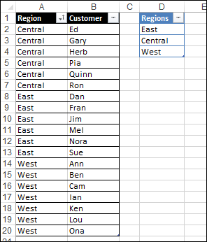
There are two lists used in this dependent data validation technique.
- The Region drop down is based on the Regions list.
- The Customer drop down shows the customers for the selected region, from the Region/Customer table
Customer Drop Down
The dependent drop down for Customer uses OFFSET, MATCH and COUNTIF to find the customers for the selected region.
- =OFFSET(RegionStart, MATCH(B2,RegionColumn,0)-1, 1, COUNTIF(RegionColumn,B2),1)
It finds the first instance of the region name, and gets customers from the next column, based on a count of the region name. In this screen shot, East is in the 8th row, and the six customers from that region would appear in the drop down.
See my website, for more details on how the formula works.

Sort By Region
For the OFFSET formula to work correctly, the lookup table MUST be sorted by the Region column. If the list is sorted by customer name, the East region list would show the wrong set of 6 names.

Check if the Regions Are Sorted
In the original version of this technique, you had to remember to sort the list by region, after making any changes to the lookup list. There wasn’t a warning system to alert you to problems.
To help avoid errors, I’ve created a new sample file, and it has formulas to check if the region names are in A-Z order.
There’s a new column (SortCheck) in the lookup table, with a formula to check the order.
- =IF(A3=””,0,–(A3<A2))
If an item is out of order, there is a 1 in the row above it. The “East” in A5 is less than the “West” in A4, so cell C4 returns a 1, instead of a zero.

Get the Total Number
In a cell named SortCheck, a formula calculates the total for that SortCheck column.
- =SUM(tblRegCust[SortCheck])
Another named cell, SortMsg, contains a typed error message that will be used in the data validation.

Show Warning in Excel Drop Down
To show a warning in Excel drop down when necessary, I changed the Customer data validation formula slightly. The IF function looks at the total, and shows the SortMsg range, if the total is greater than zero.
- =IF(SortCheck>0, SortMsg, OFFSET(RegionStart,MATCH(B2,RegionColumn,0)-1, 1, COUNTIF(RegionColumn,B2),1))
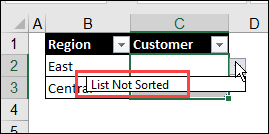
You’ll have to fix the list, before you can choose a customer name.
It’s easy to overlook a message that’s in a worksheet cell, but this error message is hard to ignore!
Other Dependent Methods
For other ways to create dependent drop down lists, go to the following pages on my Contextures site:
Get the Sample File
Get the warning in Excel drop down sample file, and see the complete instructions on my website.
______________

__________________