
Last week, I ran into problems counting Excel data with COUNTIF, and it’s Twitter’s fault! The COUNTA function can cause problems too, when it counts cells that look empty. Let’s see how to fix both of those issues.
Check for Duplicates
So, how did Twitter break my COUNTIF formula?
Every Thursday, I collect tweets for my weekly Excel Twitter post. The tweets are pasted into an Excel file, and a COUNTIF formula checks for duplicate content.
=COUNTIF(Used!C:C,H4)+COUNTIF(H:H,H4)
The result should be 1, unless there are duplicates
Last Thursday, after years without problems, one row returned a #VALUE! error, instead of a number.

New Twitter Character Limit
Recently, Twitter changed from a 140 character limit, to a 280 character limit. My workbook has a formula that checks the length of each tweet, and that one was 267 characters – the longest tweet that I’ve ever pasted into the workbook!
And yes, I have conditional formatting that highlights any tweet over 140 characters. Don’t judge me.

COUNTIF Character Limit
Unfortunately, Microsoft didn’t raise its character limits, when Twitter increased theirs, and that’s what caused the error
The COUNTIF and COUNTIFS functions can only check strings up to 255 characters. Other functions have the same limit.
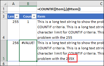
Only 255 Characters
Here’s another sample to show the problem. The 255 length works in row 4, but there is an error in row 5, which has one extra character – an X at the end.
To get a correct count, I used an old, reliable function –SUMPRODUCT, instead of COUNTIF. And since I was improving the formula, I created named ranges too, and wrapped it with an IF function.
=IF(H4=””,””,SUMPRODUCT(–(Tweets_Used=H4))
+SUMPRODUCT(–(Tweets_New=H4)))
Confusing Workaround
Later, I checked Microsoft’s COUNTIF page, and it says you can get around the 255 limit, by joining two long strings with the concatenate operator (&). That suggestion did NOT work for me though – maybe I’m missing something:
- =COUNTIF(A2:A5,”long string”&”another long string”)
Can you get that Microsoft formula to work?
Click here to download my sample file, and see more COUNTIF examples on my website.
COUNTA Counts Empty Cells
In other Excel count functions news, I’ve done a major update on my blog post about problems counting Excel data when cells look empty, but they aren’t.
In the screen shot below, data was copied from an Access database, and pasted into Excel. The COUNTA formula in cell C2 is counting those “blank” cells, even though they look empty.
![]()
Other Causes
It’s not just data from Access that creates these strange “blank” cells. They’re also created if you convert formulas to values, and some of the formulas returned an empty string (“”).
This screen shot shows that type of formula, and when pasted as values, the empty string cells are counted.
![]()
See Hidden Contents
In the update, I added a tip that lets you see something in those “blank” cells.
- On the Excel Ribbon, click the File tab
- At the left, click Option
- In the Category list, click Advanced
- Scroll down to the end of the Advanced options, and look for the Lotus Compatibility section
- Add a check mark to Transition Navigation Keys
![]()
After you turn this option on, click on a cell that looks blank, and check the Formula Bar. You should see an apostrophe there.
Remember to turn this option off later, when you’ve finished the troubleshooting.
How to Fix the Problem
My original solution was to use Find and Replace. The blanks were replaced with $$$$, and then the $$$$ were replaced with nothing.
There are instructions to manually do those steps, and there’s a macro too.

The update has 2 new solutions, thanks to the people who posted their suggestions in the comments section.
How would you fix the problem?
__________

_____________
I have a sheet that keeps track of a type of inventory. Items are arranged by page across the top (columns 2 to 65) and by individual item (rows 4 to 108). If an item is used, an “X” is placed in the cell corresponding to its page and position. Conditional formatting makes both the background and the font black so the cell is colored in, giving me a visual representation of the inventory. I use COUNTA to determine if a particular item has been used or not (blank cell = item not used). Out of 6,720 items, seven are responding as if the cell is not blank. This wreaks havoc on the inventory as these items are still available but the macro shows them as used. I have obviously hit delete until the paint is worn off the key and tried the suggestion in this blog. I have been using Excel almost since its inception and have written VBA code for over a decade. This particular puzzle has be scratching various body parts. I will be happy to send a copy of the page and the code if that helps. I would send a screen shot but there doesn’t seem to be a way to do that on this system. Thank you in advance for any light you can shed on this subject. Have a great and prosperous day.
Ed
Follow up to my earlier message, I opened a blank worksheet and ran the following code:
Sub COUNTTEST()
Dim CTR As Integer
Dim CTR2 As Integer
With Sheets(“SHEET3”)
With .Range(.Cells(1, 1), .Cells(100, 400))
.Interior.ColorIndex = 0 ‘clears all color from cells
.ClearContents ‘clears data from cells
End With
X = 0 ‘sets counter to zero
For CTR = 1 To 400 ‘columns
For CTR2 = 1 To 100 ‘rows
If WorksheetFunction.CountA(Cells(CTR, CTR2)) 0 Then ‘runs COUNTA function on cell
X = X + 1 ‘increases count when cell not blank
Debug.Print X ‘provides live result of counter
.Cells(CTR, CTR2).Interior.ColorIndex = 7 ‘colors non blank cells pink
Else
.Cells(CTR, CTR2).Interior.ColorIndex = 33 ‘colors blank cells blue
End If
Next CTR2
Next CTR
End With
End Sub
Result: 23 cells colored pink indicating they were not empty.
Still scratching …
Ed Owen
Ran into an issue with your fix for CountA when trying to count cells that are populated by a VLookup.
Using a VLookup in a different table
– wrapped in an IFError() function (to get rid of the #N/A).
– As the second field in IFError expects a value to use if there is an error in the first. Need to fill that with “something” that countA can ignore!
Trick I used to get rid of an empty string was to create a namedRange that pointed at an empty cell (a truly empty cell), and then use the named range in combination with the IFError wrapper..
Example:
=IFERROR(vlookup(A1, ‘OtherSheet’!A:B,2,FALSE), BlankCell)
where BlankCell is my namedRange (of an empty cell)
Worked like a charm to ensure CountA can count the output of a vlookup!
Thanks, Jeff, and I’m glad you found a workaround.
I’m not clear on the context in which you used it though.
If a blank cell is the 2nd argument for IFERROR, it returns a zero.
And COUNTA counts that zero, just as it would count an empty string.
Solved it for all possible scenarios. Formula to use is
=COUNTIF(range,”*?*”)+COUNTIF(range,”>0″)+COUNTIF(range,”<=0")