To see specific data in an Excel Table, you can select an item from the drop down filter in a column heading. Someone asked me if there was a way to scroll through the items, instead of opening the filter list each time. This technique uses a pivot table, which could be hidden on a different sheet, and a spin button, to go up or down in the list of items.
Scroll Through Filter Items Demo
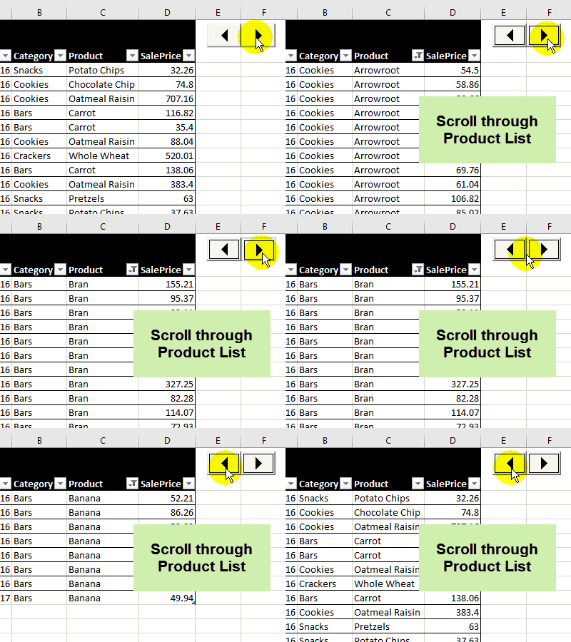
This animated screen shot shows how the scrolling technique works.
- Click the Up button, to filter by the next product in the list
- Click the Down button, to filter by the previous product in the list
- When you reach the beginning or end of the list, the next selection is “All”
Why Use Spin Buttons?
I wrote the original code for this technique long ago, to scroll through items in a pivot table report filter. Slicers hadn’t been invented yet, and the spin button was a quick way to filter a pivot table.
Now you can use Slicers to filter a pivot table or Excel table, but they take up a lot of space on a worksheet. A Spin Button is a compact way to go through a list of items, in alphabetical order.
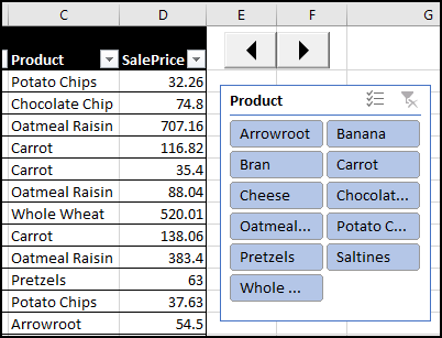
In this screen shot, you can see the size of the Spin Button, compared to a Slicer for the Product field.
How to Set Up the Spin Buttons
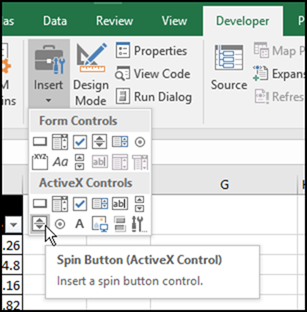
First, I added an ActiveX Spin Button on the worksheet – there are detailed instructions on the Report Filter Macros page of my website.
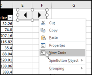
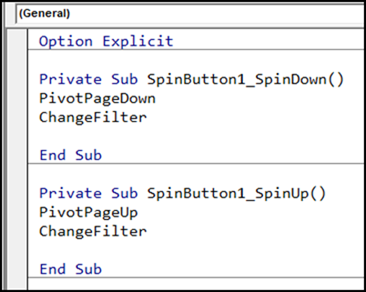
Next, I added code to the Spin Button – right-click on it, and click View Code.
Select the SpinUp and SpinDown procedures, and add two macro names in each procedure.
Create a Pivot Table
The macros will change the selected item in a pivot table’s report filter, and then change the selected item in the Excel Table’s Product column filter.
Create a pivot table, based on the Excel table that you want to filter. You can put the pivot table on the same worksheet, or on a different sheet. In the sample file, the pivot table is on the same sheet, so it’s easier to see how the technique works.
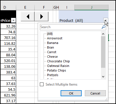
The only field in the pivot table is Product, in the Report Filter area. In the screen shot below, you can see all the items in the Product field.
Add the Pivot Table Macros
Next, you’ll add two macros – PivotPageUp and PivotPageDown. The code is in the sample file (on the modPivot module), and on the Report Filter Macros page of my website. Store this code in a regular code module.
- The code gets the current item number, then adds or subtracts 1, to get the new item number.
- It shows that item, or shows “All”, if the previous item was at the beginning or end of the list.
Add the Change Filter Macro
The final macro is named ChangeFilter, and it is stored on a regular code module. The code is in the sample file, on the modFilter module.
- This macro gets the name of the current page in the pivot table’s Report Filter.
- It selects that item in the Excel Table’s Product column, or clears the filter, if “All” is selected.
Video: Create an Excel Named Table
When you work with lists in Excel, use the built-in Table feature, to make it easy to sort and filter your data. This short video shows the simple steps
Download the Sample File
To see how the macros scroll through filter items in an Excel Table, download the sample file from my website. In the Download section on the Report Filter Macros page, look for the download named Pivot Spinner Table Filter.
The zipped file is in xlsm format, and contains macros. To test the code, enable macros when you open the file.
________________

