With the Excel VLOOKUP function, you can pull data from a specific column in a lookup table. For example, if the lookup table has Product ID, Product Name and Price, you’d use column 3 to get the price. To make your formulas more flexible, and to prevent problems, you can combine VLOOKUP and MATCH.
Why You Should Combine VLOOKUP and MATCH
There are a couple of key benefits when you combine VLOOKUP and MATCH:
- It makes the formula flexible – use one formula to pull data from different columns in the lookup table.
- It can prevent problems if new columns are added in the lookup table, or if the lookup columns are rearranged.
Video: Combine VLOOKUP and MATCH
This video shows how to combine VLOOKUP and MATCH, and there is another example, below the video.
Order Details
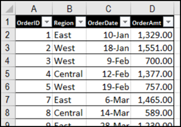
In this example, we’ll use a VLOOKUP formula to get the order details from a lookup table, based on the order ID number. Here’s the lookup table, which is named tblOrders.
Get the Details
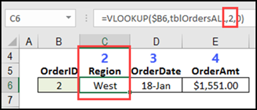
To get the details for a specific order, you could create 3 VLOOKUP formulas, with a different column number typed in each formula:
- Region: =VLOOKUP($B6,tblOrdersALL,2,0)
- OrderDate: =VLOOKUP($B6,tblOrdersALL,3,0)
- OrderAmt: =VLOOKUP($B6,tblOrdersALL,4,0)
That works, but it’s not very efficient — you have 3 formulas to maintain, instead of just 1 formula. And nobody has time for that!
The MATCH Function
Instead of figuring out which column the data is in, and then typing that column number in the VLOOKUP formula, let the MATCH function do the work for you. The MATCH function finds the position of an item in a list, and returns that position number.
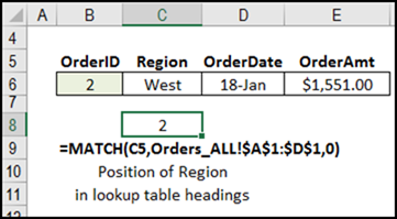
For example, if the MATCH function looks for “Region”, in the lookup table heading cells, the result is 2.
=MATCH(C5,Orders_ALL!$A$1:$D$1,0)
Cell C5 has the heading “Region”, and that is a relative reference. Later, if the formula is copied to the right, it will refer to the headings in D5 and E5.
Replace the Typed Number
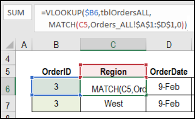
To add the MATCH function to the VLOOKUP formula, just replace the typed column number
=VLOOKUP($B6,tblOrdersALL,2,0)
with the MATCH formula:
=VLOOKUP($B6,tblOrdersALL,MATCH(C5,Orders_ALL!$A$1:$D$1,0),0)
Copy the VLOOKUP Formula Across
Now, instead of needing a different formula in each column, you can copy the formula across, and use the same formula in all the columns. In each column, the MATCH function’s first argument (C5) will change, and refer to the heading cell in that column.
Keep the Headings the Same
For this technique to work correctly, the headings on the VLOOKUP sheet have match the lookup table headings exactly.
- In my sample file, the VLOOKUP heading cells are linked to the lookup table heading cells.
- If you can’t use links, copy and paste the headings from the lookup table, to be sure they’re exactly the same.
Get the Sample Workbook
Go to the VLOOKUP page on my Contextures website, to get the sample workbook. In the Download section on that page, click the link to Sample File #1.
The zipped file is in xlsx format, and it does not contain any macros.
_____________________
_________________________________


