If you need to get a product price in Excel, you can use VLOOKUP or INDEX/MATCH to get the price from a lookup table, based on a product code. But what if you have two pieces of information, such as a product name, and a size, and you want to find the price based on that information? How can you do an Excel lookup with two criteria?
Use INDEX and MATCH
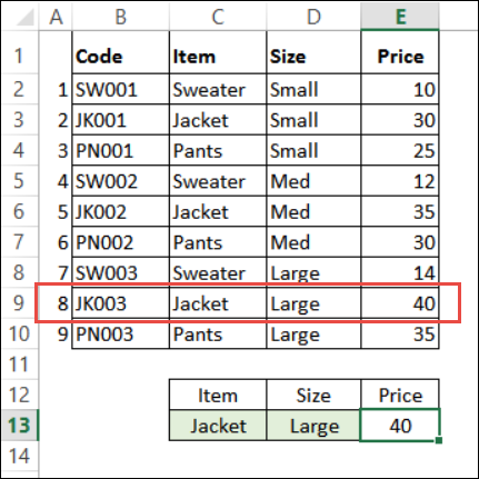
A few years ago, I posted an example that shows how to check multiple criteria with INDEX and MATCH. There is a lookup table with columns for product code, item name, item size and the price.
Below the table, I entered “Jacket” as the item name and “Large” as the size. In cell E13, I need to find the price for that item and size.

Find the Row That Matches
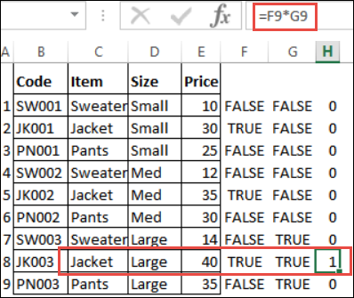
To find the price, you have to check each row, with two tests:
- Is the item name the same as the item in cell C13? (TRUE or FALSE)
- Is the item size the same as the size in cell D13? (TRUE or FALSE)
If you multiply the result of those two tests in each row, the result is a 1 or a 0. The row with 2 TRUE results has a 1, and all other rows, with one or two FALSE results, show a zero.
With those formulas on the worksheet, you could use the MATCH function to find the 1 in column H, and return the price from that row.

Do the Tests in a Formula
Instead of adding extra columns to the worksheet, you can use an array-entered formula to do the tests, and the multiplication.
Here is the INDEX/MATCH formula that for this example.
=INDEX(E2:E10,MATCH(1,(C13=C2:C10)*(D13=D2:D10),0))
NOTE: This is an array-entered formula, so press Ctrl + Shift + Enter, instead of just pressing the Enter key.
The MATCH function will find the 1 in that array of results, and the formula returns the price in that row.
Video: Excel Lookup With Two Criteria
First, this video shows how a simple INDEX / MATCH formula works. Then, the formula is changed, to work with multiple criteria. Simple formulas on the worksheet show why the MATCH function can find the correct row.
The timeline is below the video, and you can download the sample file to follow along.
0:00 Introduction
0:26 Lookup with One Criterion
1:52 Test Each Criterion
2:22 Test With a Formula
3:26 Multiply the Results
4:03 INDEX / MATCH Formula
5:20 Check the Formula
5:57 Get the Sample File
Get the Excel Lookup With Two Criteria Sample File
Visit the INDEX/MATCH page on my website to get the Excel Lookup With Two Criteria sample file. This is Example 4 in the sample file.
_________________
