You can make an interactive dashboard in Excel, even if you can’t use macros, or prefer to avoid them. Select a chart or chart data from a drop down list, and the selected item will instantly appear on the dashboard – no macros required.
Video: Choose Dashboard Items from Drop Down List
This video shows how to set up a dashboard where you can choose between 2 items – a chart, or the chart’s data.
The steps below are for a similar 4-item version. Download the sample file (link below), to follow along with the video.
Choose Dashboard Items from Drop Down List
See how to build this dashboard, follow the steps below, and download the sample file to see the completed version.
Name That Range
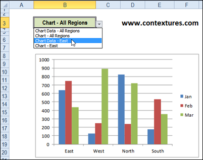
In the screen shot above, “Chart Data – East” is selected in the drop down list, and that data will appear on the dashboard, replacing the current data.
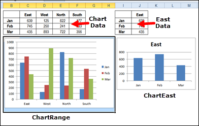
There are 4 choices in the drop down, and on a separate worksheet (ChartInfo), there are four matching ranges, shown below.
- ChartData
- EastData
- ChartRange
- ChartEast
The contents of the selected range will appear on the dashboard.
Items for the Drop Down List
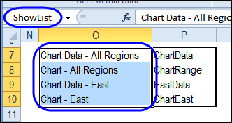
The list items for the drop down are stored in a range named ShowList, on the ChartInfo sheet.
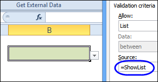
Then, on the dashboard sheet, a data validation list is based on the ShowList name.
Create a Lookup Table
In the column to the right of the drop down list items, the matching range names for each item are entered.
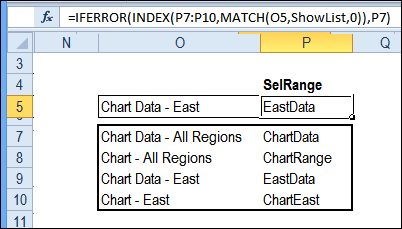
Above the lookup table, cell P5 is named SelRange, and it has an INDEX/MATCH formula that returns the range name for the item selected in the drop down list:
=IFERROR(INDEX(P7:P10,MATCH(O5,ShowList,0)),P7)
The Chart Data – East item was selected, and its range is named EastData
Add a Linked Picture
Next, a named formula — ShowChart was created. It uses the INDIRECT function to return the range from the SelRange cell:
=INDIRECT(SelRange)
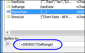
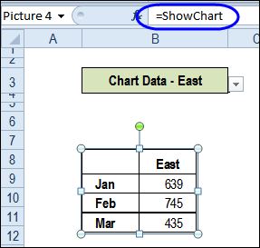
Finally, on the dashboard sheet, a linked picture was added, and its link was set to ShowChart. Now, when you select an item from the drop down list, the linked picture changes, to show the range that matches the selected item.
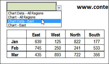
In the screen shot below, Chart Date – East was selected, so the EastData range is shown.
Download the Sample File
To see how the interactive dashboard works, you can download the sample file from the Excel Sample Files page on my Contextures website. In the Charts and Graphics section, look for CH0002 – Show or Hide Excel Chart. There are 3 versions of the file, so download the ones that you need:
- Excel 2003,
- Excel 2010 (2 item drop down)
- Excel 2010 (multi-item drop down)
___________________
