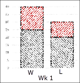
Last weekend, I helped someone who needed a chart for a fantasy football league, to show the highest and lowest win/loss scores for each week. To help explain what it should look like, they posted a picture of a hand drawn chart, similar to the picture below.
By the way, I created the sketch in Excel, by using the Marker option, in the Artistic Effects. Who knew that Excel was so artistically talented?
Set Up the Data
The win/loss data was set up with a separate column for each week, and rows for the win and loss highs and lows.
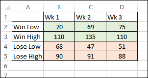
To create the type of chart that’s in the sketch, we’ll need to build a clustered stacked column chart. Blank rows and columns need to be added, and the numbers have to be staggered, with the Win and Loss numbers in separate columns.
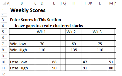
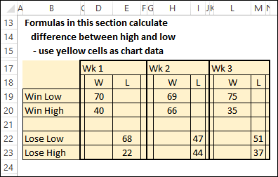
The difference between the high and low scores needs to be calculated too, so the High amount is correctly shown. I also added a “W” or “L” heading to each column of scores, so the chart will be easier to understand.
Create the Chart
The yellow cells, in the screen shot above, are used as the source for the chart.
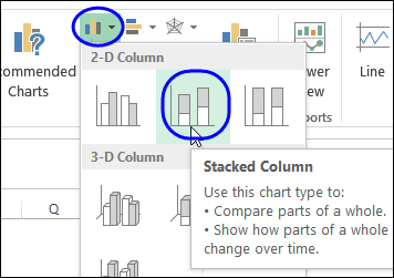
On the Ribbon’s Insert tab, click Column Chart, then click the Stacked Column option
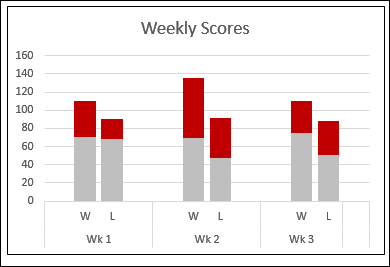
After the chart is created, change the formatting so the gap is smaller, and the High and Low series have the colours that you want.
In the screen shot below, you can see the chart that I created.
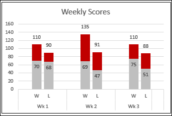
If you want the actual High scores to appear, copy the Win High label and data (row 7), and Lose High label and data (row 11), and paste them into the chart. Then, change the 2 new series to Line Charts.
Then, add data labels to the Line Charts, to show the High scores, and add data labels at the Inside End for the Low scores.
Clustered Stacked Chart Utility
If you don’t have the time or patience to arrange your data and create your own Clustered Stacked Column chart, Jon Peltier has an Excel Chart Utility. that will make the job easier for you.
You can see how it works in this video, or watch on YouTube: Create a Cluster Stack Chart With Excel Chart Utility
Download the Sample File
To see how the data is set up, and view the completed chart, you can download the sample file from my Contextures website. On the Sample Excel Files page, go to the Charts section, and look for CH0010 – Show High and Low in Clustered Stacked Chart. The zipped file is in xlsx format, and does not contain macros.
_________________________
