I like to color data entry cells, so they’re easy to spot on an Excel worksheet. If you know that you should type a value in every blue cell, it’s quicker, and safer, to fill in a worksheet.
Recently, I was asked how to color a specific number of data entry cells, based on a number that someone selected from a drop down list. So, instead of manually coloring the data entry cells, I used conditional formatting to color them.
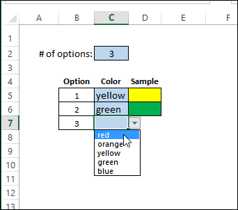
In the screen shot below, 3 was selected in cell C2, so 3 data entry cells are blue, in cells C5:C7.

Select a Color
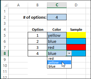
Another feature in this workbook is the drop down list of colors in column C. After you select a color, a sample of that color appears in column D. Select a different color from the drop down, and the sample color will change.
This is also done with conditional formatting – no macros required. There are 3 colors set up in the sample file, with a separate rule for each color. You could set up more rules if necessary.

Detailed Instructions
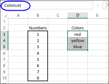
On my website, you can follow the step-by-step written instructions, to see how to set up the workbook, with lists in named ranges, and add the data validation and conditional formatting. Or, watch the video below, if you’d prefer to see me build the workbook, rather than read the steps.

Video: Conditional Formatting Colors
To see the steps for setting up the workbook, and adding drop down lists and conditional formatting rules, please watch this video tutorial.
Or Watch on YouTube: Color Excel Data Entry Cells With Conditional Formatting
Download the Sample File
To see how the conditional formatting works, you can download the sample file from my Contextures website. The zipped file is in xlsx format, and does not contain macros.
_______________________
